Tornadoes
A tornado (also called a twister) is an extreme meteorological event that can be very dangerous for populations and can cause a lot of damage. According to the World Meteorological Organization, tornadoes kill between 300 and 400 people each year and including 150 only in the United States. Indeed, some regions are more vulnerable and more exposed to tornadoes. But before explaining their distribution around the world, we need to understand how they formed.
Table of contents
- How are tornadoes formed
- What causes a tornado to stop?
- Categories of tornadoes (Enhanced Fujita scale)
- Types of tornadoes
- What looks like a tornado but isn’t?
- Where do tornadoes occur in the world?
- Tornado Alley
- Dixie Alley
- Hoosier Alley
- Carolina Alley
- The 10 most deadliest tornado in the world
How are tornadoes formed
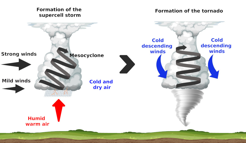
Tornadoes form only under very precise conditions. Most of the tornadoes form in a supercell thunderstorm. These storms are very powerful thunderstorms that form essentially in summer.
Indeed, the sun warms the ground, giving a warm and wet air parcel. This air that escape from the ground is warmer and so less dense. As a result the air parcel will rise.
The air parcel, by rising up, will meet a cold and dry air. The wet air parcel will condense and form a cumulus cloud. If the air above is cold and dry enough and they air that rise warm and wet enough, it will continue to raise until the tropopause to form a cumulonimbus. This cycle is the standard cycle of a thunderstorm, but we still don’t have a supercell.
To get a supercell thunderstorm, there needs to be a wind speed variation (more quickly with the altitude) or directions variation with the altitude. This effect is the so called wind shear. This will induce a horizontal rotation inside the cloud. This horizontal tube will be pushed to the vertical by the ascending air of the cumulonimbus. This gives finally an inclined rotating tube of air inside the cumulonimbus, which is called a mesocyclone. By then the full cloud starts to rotate, which by now can be called a supercell thunderstorm.
These supercell thunderstorms can stay active for hours with heavy rain, hailstone and thunders.
To get a tornado from these supercell thunderstorms, we need more powerful winds. Inside the cloud, the rain cools the air, which become more dense and they go down to the ground. These downward currents encircle the mesocyclone and force him to the vertical. A small cone, called tuba, form under the cumulonimbus. The winds accelerate until the ground surface and when the tuba touch the ground, we get a tornado with winds that can flow with a speed of 400km/h (250 mph).
Not every supercell thunderstorms produce tornadoes. Only around 20 percent of all supercell thunderstorms produce tornadoes.
What causes a tornado to stop?
The phenomenon is fading when the balance between rising and falling air is no longer maintained or when the tornado meets a relief.
Categories of tornadoes (Enhanced Fujita scale)
Tornadoes are categorized by order of their seriousness of the damage that they cause. The first scale used for this classification was the Fujita scale, also called the Fujita-Pearson Scale or F scale. This scale was established in 1971 by Ted Fujita and Allen Pearson.
It is important to note that this classification is not based directly on the wind speed, but rather on the damage caused by the tornado. The categories of tornadoes are determined afterwards the tornadoes is done.
The Fujita had originally 6 categories (from F0 to F5) which is add 7 theoretical categories never met en that go from F6 to F12.
Average wind speed in the tornado, 10 m altitude above flat ground, are given for indication (harder short time winds are possible). These wind speeds are indicative because no direct relation between wind speeds and damages have been done.
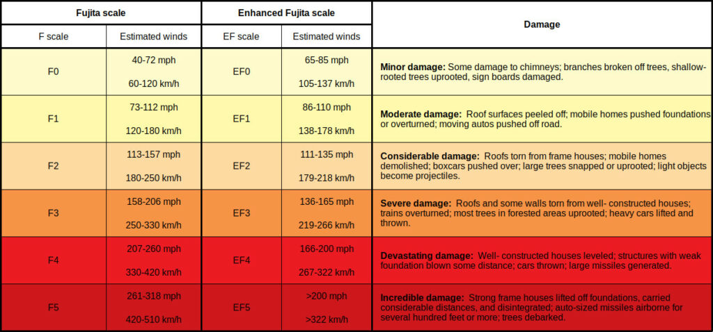
The Fujita scale had received some critics because it didn’t take into account some factors like the quality of the materials of the buildings, not enough indicators,… Because of this, an Enhanced Fujita scale has been released in 2007. This new scale has 28 indicators, which helps to take into account much more types of building and quality of buildings. It also uses an estimation of speeds obtained by meteorological radars. This new scale also helps to categorize tornado in every part of the world more accurately.
The 2 scales are similar and have the same categories. Only the way to determine the intensity of the damage is different and also the speeds of the winds to produce these damages are different. Indeed, the meteorologist had the impression that the winds in the first scale were too high for the damage caused. Indeed, the total devastation of the F5 was caused following the scale by winds of 420 km/h (261 mph) and the new scale determine the speed necessary to be 322 km/h (200 mph).
Types of tornadoes
Tornadoes are usually distinguished in supercell and non-supercell, with therein different subtypes.
Supercell tornadoes
These tornadoes are the most common and often the most dangerous. In function of their shape and size, we can distinguish different subtypes. Tornadoes that lived for a certain time may transit from one type to another as it changes in size and shape during its life.
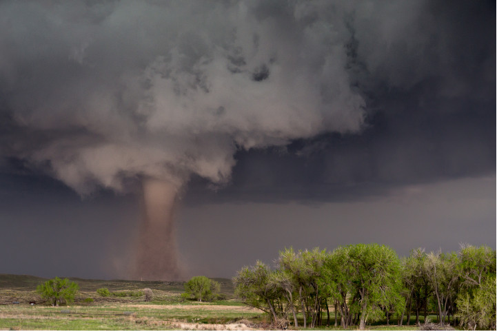
Rope tornado
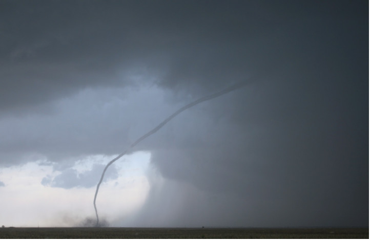
They have the shape of a rope and they are the most common types and the smallest tornadoes. Most tornadoes begin and end their life as a rope tornado. Some also stay in this type and only last a few minutes.
Although they are the smallest of all the tornado, they are still dangerous and some of them get more intense as they narrow and tighten.
Cone tornado
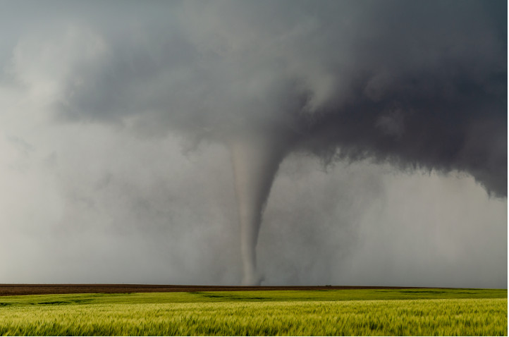
This type of tornado has the “typical” conical shape of a tornado with a wider base than the robe tornadoes and they are much wider on the side touching the thunderstorm.
The cone tornadoes have a wider footprint on the ground and so they can leave a larger trail of destruction.
Stovepipe or cylinder tornado
Theses tornadoes are similar to the cone tornado, but the width on the ground is similar the width at the base of the thunderstorm.
Wedge tornado
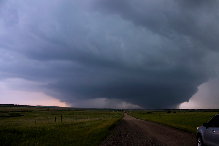
Wedge tornadoes are wider than they are tall (at least as wide as their height cloud-ground). The width is around 1 km (0.6 mile) and more. Wedge tornadoes are usually classified EF-3 or more. These tornadoes leave huge destruction trails.
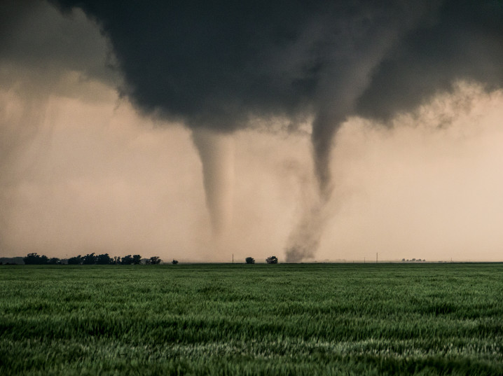
Satellite tornado
A satellite tornado is a tornado located around a main primary tornado and is interacting with the same mesocyclone. Satellite tornadoes are apart from the primary tornado and so they are different then multiple vortex tornadoes. These types of tornadoes are not common. The satellite tornado and the primary tornado are called a couplets.
Multiple vortex tornado
A multiple vortex tornado is a tornado with several vortices (called subvortices or suction vortices) circling around or inside and as a part of the main vortex. The subvortex can produce localized area of higher winds than the main circulation.
This type of tornado is difficult to observe because of the dirt and debris carried upward. They are visible when the tornado form or when the condensation and the debris are balanced. They form usually in the lower part of the tornado vortex where the tornado makes contact with the surface.
Non-supercell tornadoes
Non-supercell tornadoes are not linked with a storm rotation and are rather created by a vertically spinning parcel of air occurring near the ground. These tornadoes cause less damages than the supercell tornadoes.
Landspout
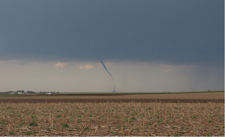
Landspout is a narrow rope-like condensation funnel that form while the thunderstorm cloud is still growing. They are formed by a vertically spinning parcel of air occurring near the ground. These tornadoes are weaker than the one caused by supercell, but they can still cause serious damage (until EF2).
Waterspout
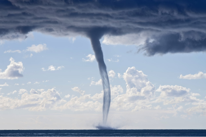
Waterspout are like landspout, but they form above water. A few of the waterspout are stronger and can be caused by a supercell thunderstorm. But the big majorities are non-supercell tornadoes. Sometimes they can hit the ground and then become a land tornadoes.
What looks like a tornado but isn’t?
Some phenomenon looks like tornadoes because they have the same rotation characteristics, but they are not considered like tornadoes. Indeed a tornado needs to be linked with a storm event. Below is a list of events that looks like tornadoes, but that are not.
Gustnado
Gustnado (or gust front tornado) are small vertical swirl associate with a gust front of a storm system. They look like real tornadoes, but they are not connected to the base of the cloud and so they are not considered as tornadoes.
Dust devil

Dust devil are also composed of a vertical swirling column of dust, which make them look like a tornado, but it is not a tornado because there is no link with a cloud. They form under clear skies and hot day. They are formed by a strong convective updraft from the warm air on the ground surface and low level wind shear.
They have diameters from 1 centimeter to 10 meters and a vertical extension that goes from a few meters to more than 1000 meters.
They last only for a few minutes and they can be as strong as the weakest tornadoes. So they can cause minor damages.
Dust devil is the common name, but it has local names like willy-willies in Australia
Fire whirls
Fire whirls are not common and usually very weak, but it can be as strong as an EF3. They are associated with wildfires and the large difference of temperature between the fire on the ground and the cooler air in altitude causes the air to rise. The rising air and the wind circulation above the ground create the rotation.
Steam devils
Steam devils are very rare to observe. They are rotating updraft of steam or smoke. They are not linked with high wind speeds (the rotation is at a speed of only a few rotations per minutes). They form mostly from smoke from power plants, but it can also form above hot springs, deserts, water areas, …
Where do tornadoes occur in the world?
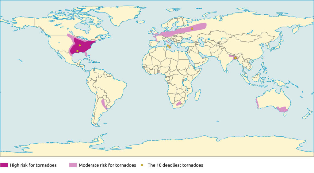
Tornadoes occur in different regions of the world, but some of them are more hits.
The United States are hit by the highest number of tornadoes and they are of very high intensity. Between 800 and 1300 tornadoes are registered in the US each year and around 20 of them are from the EF4 or EF5 category.
| Rank | States | Annual average number of tornadoes by 10,000 sq miles (25 900 km²) |
|---|---|---|
| 1 | Florida | 12.2 |
| 2 | Kansas | 11.7 |
| 3 | Maryland | 9.9 |
| 4 | South Caroline | 9.8 |
| 5 | Illinois | 9.7 |
| 6 | Mississippi | 9.2 |
| 7 | Iowa | 9.1 |
| 8 | Oklahoma | 9 |
| 9 | Alabama | 8.6 |
| 10 | Lousiana | 8.5 |
| 11 | Arkansas | 7.5 |
| 12 | Nebraska | 7.4 |
| 13 | Missouri | 6.5 |
| 14 | North Caroline | 6.4 |
| 15 | Tennessee | 6.2 |
| 16 | Texas | 5.9 |
| 17 | Minnesota | 5.7 |
The highest density of tornadoes in the world is located in Florida and they are mostly of low intensity in this region.
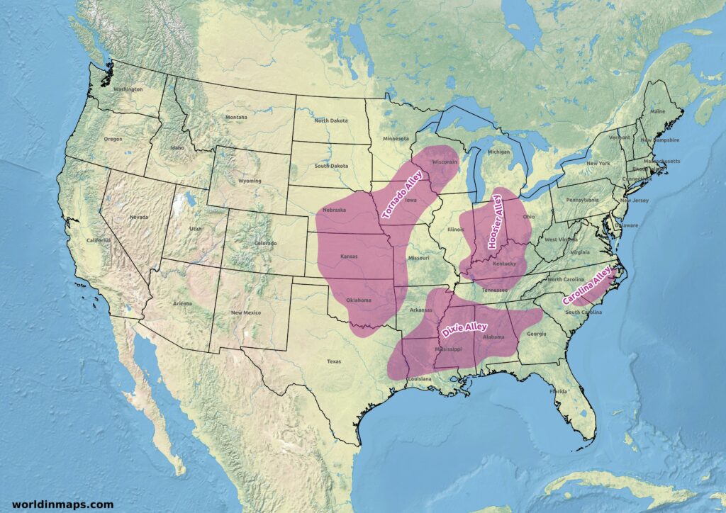
But the most active area is the Basin of the Mississippi River and the Great Plains in the United States. The tornadoes are there generally very powerful. It is for this reason that the states of Texas, Oklahoma, Kansas, Nebraska, Arkansas, Missouri, Iowa and Wisconsin were given the name Tornado Alley witch one third of the Tornadoes of the United States. The next chapters will detail the four main United States Alleys (Tornado Alley, Dixie Alley, Hosier Alley and the Caroline Alley).
Other parts of the world are also hit by tornadoes. In Africa, they can be found in South Africa.
In South America they happen in some regions of Argentina, Paraguay and the south part of Brazil.
In Europe, they are more common in the plain of northern Europe, especially in Germany and Poland. But in terms of density it is in the Netherlands that they are the highest with 20 tornadoes per year and a density of 0,00048 per square kilometer. Then it is followed by the United Kingdom and its 33 tornadoes. Mostly they are from very low intensity and they are mostly EF1. The European Tornado Alley is located between the Benelux (Belgium, Netherlands and Luxembourg) and Germany.
Tornadoes also happen in Australia and New Zealand.
Finally, they are also very common in the Delta of the Gange in Bangladesh. They are as often and strong as in the United States and count more dead each year than in the United States. But there is less mediatization about them.
Urban and rural areas are both touched by tornadoes. Some big cities report numerous tornadoes in their metropolitan area like Miami, Oklahoma City, Dallas, Dhaka, …
The reporting number of tornadoes is strongly depending on the distribution of the world population. For example, Canada report 80 to 100 tornadoes each year, but big areas of Canada are sparsely populated and the real number is probably much higher.
Tornado Alley
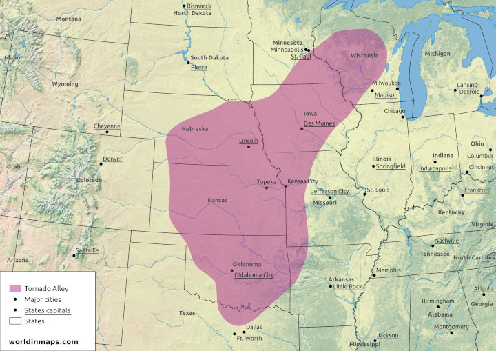
The Tornado Alley refers to a central region of the United States, covering several states or parts of states, where tornadoes are frequent.
There is not exact delimitation of the Tornado Alley, and the boundaries depends on the statistics used.
The Tornado Alley totally include the Oklahoma, the Kansas and the Iowa states. It covers also the northeast of the Texas, the northwest of the Arkansas, the west of the Missouri, the east of the Nebraska, a little part of the south of the South Dakota, the southeast of the Minnesota, a little part on the northwest of the Illinois and finally the central part and the southwest of the Wisconsin.
Although tornadoes occur in every region of the United States, they are much more frequent in this region located in the great plain, between the Rocky Mountains and the Appalaches where the condition for tornadoes are optimal.
Indeed, the Tornado Alley is located at the meeting of the continental cold air parcels coming from the Canadian Prairies, with the dry and hot air from the desert of Sonora, the hot and wet air coming from the Gulf of Mexico and finally with high variation of winds with altitude because of the presence of a Jet Stream.
Tornadoes can occur all the year around, but their frequency varies during the tornado season. Indeed the Tornado Alley trend to switch to the north with the warming of the temperature, from spring to summer, and on the opposite to the south when the temperature become colder in autumn.
The consequence of this Tornado Alley is that in its center part the building standards are more strict. With for example reinforced roof, tornado shelters, …
Dixie Alley
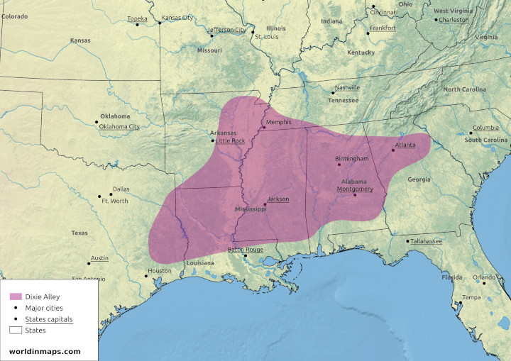
The Dixie Alley is the name given to a region of the United States where a very high number of tornadoes happen each year and of very high intensities.
The Dixie Alley includes much of the region of the lower Mississippi. It includes the following states: Mississippi, Louisiana, the east of Texas, the east of Arkansas, the southwest of Tennessee, the Alabama and the north of Georgia.
This region is under favorable condition to produce tornadoes, which explain their high numbers. Indeed, it has the same condition as the Tornado Alley. The region is under the cold continental air coming from the north and the hot and wet air from the Gulf of Mexico. This creates a very unstable condition. The cold air flowing to the southeast uplift the hot air. These hot air parcels continue their uplift and the humidity condense to create storms with very height vertical extension, the so called cumulonimbus clouds.
From autumn to spring, the region is under winds that are from different directions and intensity with the altitude, because of the presence of a Jet Stream. This wind shear will create the supercell thunderstorms that will be able to give tornadoes. In the summer the Jet Stream moves to the north.
The pic of intensity of tornadoes in this region is around May and with a second wave in October and November. But tornadoes can be seen all the year around. Which make them very dangerous in this region because a tornado can still happen outside the tornado season, when people’s vigilance is lower.
Indeed, this region produces less tornadoes then the Tornado Alley, but there is more dead in this region each year than in the Tornado Alley. Another reason is that tornadoes are very powerful in this region and that they travel long distances in an area of high population density. According to the National Centers for Environmental Information, Texas, Alabama, Mississippi, Arkansas and Tennessee are States on top of the ranking of the number of deaths from tornadoes between 1950 and 2006. Another factor is that the supercell thunderstorms also happen during the night, which can surprise people in their sleep. Finally the storms produce very high precipitation, which make the tornado difficult to see.
Hoosier Alley
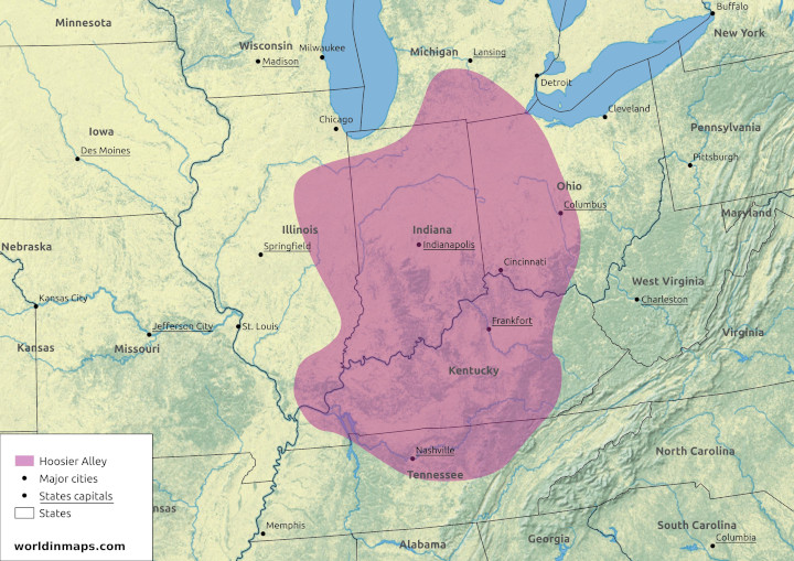
The Hoosier Alley is the third most active area in the United States for tornadoes. This alley is centered on the Indiana and includes the east of Illinois, the Kentucky, the north of Tennessee and the west of Ohio. Like for the Dixie Alley these storms are fast moving and with a lot of rain, which make the tornadoes difficult to see.
Carolina Alley
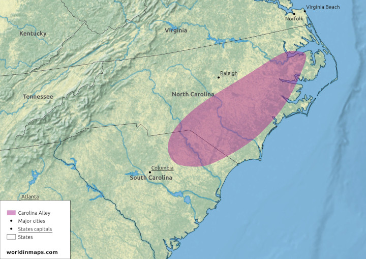
The Carolina Alley is the fourth most active area for tornadoes in the Unites states. This alley is located in North Carolina and the northeastern of South Carolina.This alley is also concerned with fast moving storm and heavy rains.
The 10 deadliest tornado in the world
| Rank | Name / location | Country | Date | Deaths |
|---|---|---|---|---|
| 1 | Daultipur and Saturia | Bangladesh | 26 April 1989 | 1300 |
| 2 | Tri-State Tornado | US | 18 March 1925 | 695 |
| 3 | Manikganj, Singair and Nawabganj | Bangladesh | 17 April 1973 | 681 |
| 4 | 1969 East Pakistan Tornado | Bangladesh | 14 April 1969 | 660 |
| 5 | Grand Harbour at Valletta | Malta | 23 September 1551 | 600 |
| 6 | Magura and Narail Districts | Bangladesh | 11 April 1964 | 500 |
| 6 | Sicily | Italy | 8 December 1851 | 500 |
| 6 | Madaripur and Shibchar | Bangladesh | 1 April 1977 | 500 |
| 9 | Belyanitsky, Ivanovo, and Balino | USSR | 9 June 1984 | 400 |
| 10 | Natchez, MS | US | 6 May 1840 | 317 |
Global atmospheric circulation
Winds tend to change daily in function of the weather, but there is some regularity in the movement of the air masses. The global atmospheric circulation pattern explains this regularity of the air movement around the earth.
Table of contents
- Causes of the global atmospheric circulation
- What are the 3 types of atmospheric circulation cells?
- Walker circulation cell
- The Coriolis effect
- Jet stream winds
- Trade winds, westerlies and polar easterlies
- Intertropical convergence zone (ITCZ)
- Seasonal change in the atmospheric circulation and precipitation
- The atmospheric circulation cells and climatic zones
Causes of the global atmospheric circulation
The movement of the air masses on the earth’s surface is strongly depends on the temperature. Indeed, when the air is warmed it became less dense and it is gaining altitude. This form what is called a depression in meteorology. On the opposite, when air is cold, it is more dense and it tends to go down. This last system is called an anticyclone in meteorology.
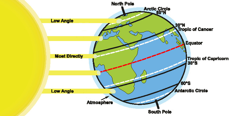
To understand the global pattern of the atmospheric circulation, we need to take a look to the variation of the temperature on the earth. The distribution of the temperature on the earth is depending on the solar radiation. Indeed the sun warms the earth differently in function of the distance of the equator. At the equator, the sun is nearly vertical and intense. The most we move to the pole, how more the rays are inclined and therefore less intense. As a result, the equator receives more incoming solar radiation then the poles.
The earth emits back outgoing longwave radiation and a part of the solar radiation. These outgoing emissions are higher on the pole than at the equator. The net balance between outgoing and incoming is negative at the pole and positive at the equator. The global atmospheric circulation and the ocean circulation are responsible to redistribute the thermal energy at the earth’s surface. This atmospheric redistribution is divided into 3 different cells.
What are the 3 types of atmospheric circulation cells?
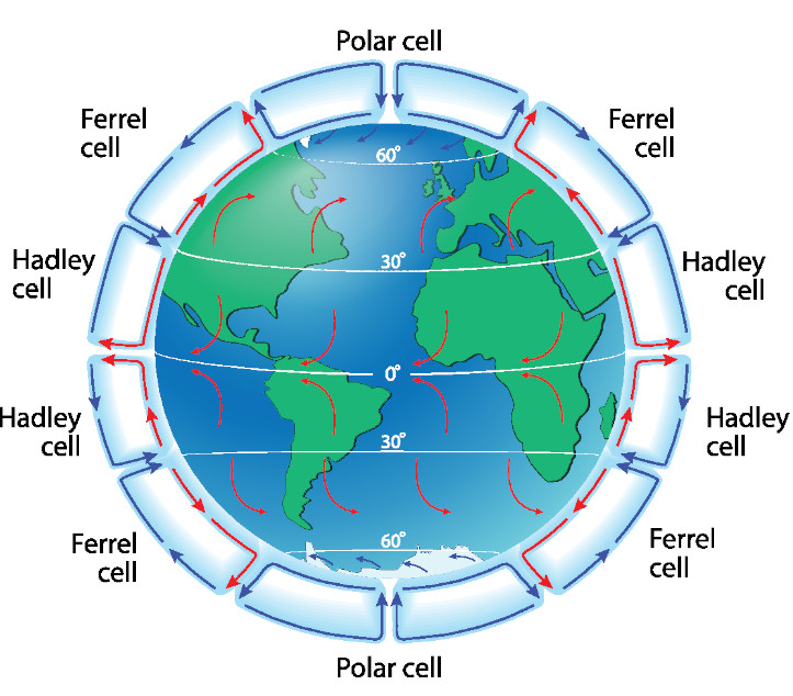
Hadley cell
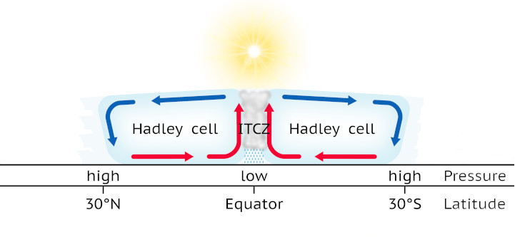
As explained in the previous chapter, the solar radiation is the highest at the equator. The result is a hot and wet air. This instable air masses create convection. Indeed, when the air gets hotter it expands and therefore becomes lighter. Because the air is lighter it will take altitude, which cause wind to replace the air that go up with air that come from the sides.
This convection causes low pressure zones near the equator and cumulonimbus clouds form with very high vertical extensions, which bring daily afternoon rain. These clouds stop their vertical extension at the tropopause (the boundary between the troposphere and the stratosphere with an altitude varying from around 8 km (25,000 ft) at the pole to around 18 km (60,000 ft) at the equator). Indeed, this boundary marks the inversion of the temperature rate. At this boundary, the temperature stop to become colder with the altitude and the air is dry once this limit is passed. As a result, it stops the vertical extension of the cumulonimbus cloud at an altitude of around 18 km (60,000 ft) at the equator.
Because the air is blocked at the tropopause, it starts to move to the sides towards the poles. While moving to the tropics, the air cools and it becomes denser. Finally, it is so dense that it descends around the tropics (latitude of 30°). This creates high pressure zones around the tropics with dry air. Finally, the air masses flow back to the equator at the surface of the earth.
This type of cell is at the number of 2, one on each side of the equator. This cell type is the biggest of the 3 types.
Polar cell
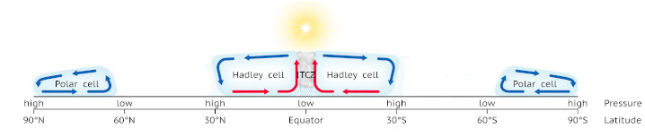
The Polar cell is the most little of the 3 types of cells. This cell is located at each pole.
At the pole the air is cold and dense, by consequence, it descends to the ground. Then it flows to a latitude of around 60° North for the cell at the North pole and South for the cell at the South pole. While moving to this latitude the air start to warm and it rises in the atmosphere at around 60° latitude to go back to the pole.
Ferrel cell
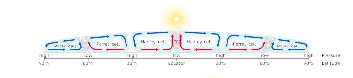
This cell is located between the Polar cell and the Hadley cell, in other word between the latitude of around 30° and 60°. Unlike the 2 other cells, this cell is not driven by temperature. This cell exists only because of the existence of the other cells. This cell is also different because the circulation of this cell is in the opposite direction than the Polar and Hadley cells.
Walker circulation cell
Next to the 3 majors cells defined above and that divide the earth from pole to pole, there is the Walker circulation cell which, on the opposite to the other cells, is circum-equatorial. In other words, this cell is located along the equator, and so perpendicular to the 3 major cells. This cell is caused by the intensity contrast of heating between the continents and the oceans, which create convection and subsidence zones along the equator. The Walker cell is the convection and subsidence system located in the Pacific Ocean.
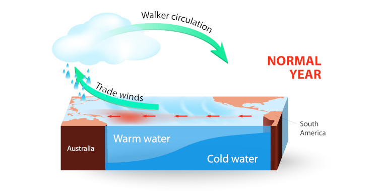
The Walker cell is more exactly located between Australia and South America. The trade winds blow from East to West and brings Warm ocean water towards the low pressure system located in Indonesia and Australia. On the opposite we have on the coast of South America an upwelling of deep cold water and the cold current of Humbold (also called the Peru Current) with as a consequence a high pressure system. This results in a dry weather on the west coast of South America.
The accumulation of warm ocean water along Indonesia and Australia lead to active convection with heavy rainfall and thunderstorms. The air parcel raises until the troposphere and then flows back and cools to South America, to the subsidence area located on the high pressure system along the coast of South America.
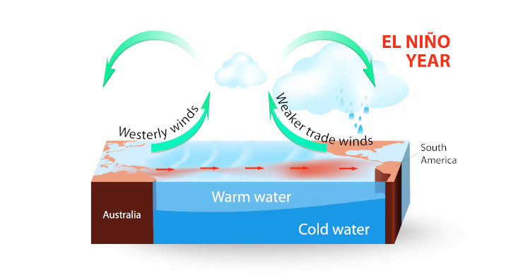
The cycle above describes the normal cycle of Walker. But during a few months of the year the trade winds may be weak, which allow the pilled hot water of the western Pacific to move to the eastern Pacific. This change totally the oceanic current and the atmospheric circulation in the area. By consequence, it blocks the upwelling of cold water on the coast of South America and the water become more warm. This phenomenon starts a bit after Christmas and finish in April. This has consequence on the fish activity because with the disappearing of the upwelling the nutriments for the fish disappears and the fish also with them. Finally the coast, that is normally very arid, is also affected by rainfall. This modification of the cycle of Walker is named ENSO (El Niño – Southern Oscillation).

On the opposite, we have the La Niña which is an amplification of the trade winds, which push further the warm ocean water on the western pacific. This allows the deep cold water to occupy a bigger part of the eastern Pacific. The consequence on the coast of South America is a better fishing activity, but also a more long dry weather. It also gives colder winter in North America because the warm water is pushed further away in the western pacific. It gives also more hurricane in the Atlantic ocean.
The Coriolis effect
The Coriolis effect is the consequence of the earth rotation. Indeed the earth makes a full turn in 24h, but a point on the pole have 0 km (0 mi) to do in 24h. On the opposite, a point at the equator have 40 074 km (24,901 mi) to do in 24h. In the tropics of the Cancer and the Capricorn the length is 36 814 km (22,875 mi). By consequence a point will move at a speed of 1 670 km/h (1,037 mph) at the equator and 1534 km/h (953 mph) at the tropics.
These differences in speed have a consequence on the moving air in the atmosphere. In the northern hemisphere the winds are deviated to the right and in the southern hemisphere the winds are deviated to the left.
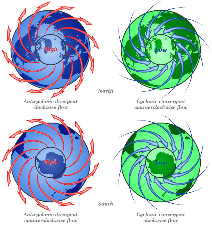
The Coriolis effect explains why the air in a low pressure system is counterclockwise in the northern hemisphere. Indeed, this deflection twists the air flowing inwards to right, creating a counterclockwise swirl of winds.
In a high pressure system, the air flows outward and the deflection has as result a clockwise rotation.
In the southern hemisphere it is the opposite and so the air flows clockwise for low pressure systems and counterclockwise for high pressure systems.
Jet stream winds
The Coriolis effect is responsible for the creation of narrow bands of very strong winds called jet stream. These winds are very strong and can have maximal speed above the 360 km/h (225 mph). This winds are located at front area between the different cells.
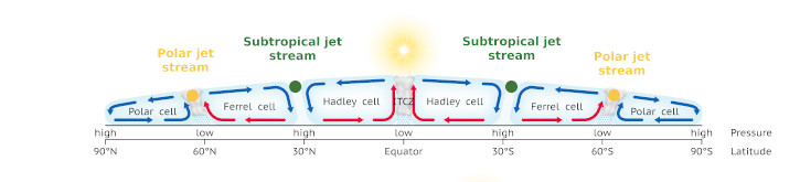
The subtropical jet streams are located between the Hadley cells and the Ferrel cells. They mark the limit between temperate area and more hot areas. They are located around 12 and 15 km of altitude (40,000 and 50,000 ft) and their position vary in function of the seasons.
The polar jet streams are located between the Ferrel cells and the Polar cells at an altitude of 11 and 13 km (36,000 and 40,000 ft). They delimit the temperate areas of the cold areas. These jet streams are located at the so called polar front and they are the result of the contrast of temperature across the polar front. More is the contrast of temperature more strong is the jet stream. As a consequence, these jet streams are stronger in the winter than in the summer. Indeed the difference of temperature is stronger in the winter.
Trade winds, westerlies and polar easterlies
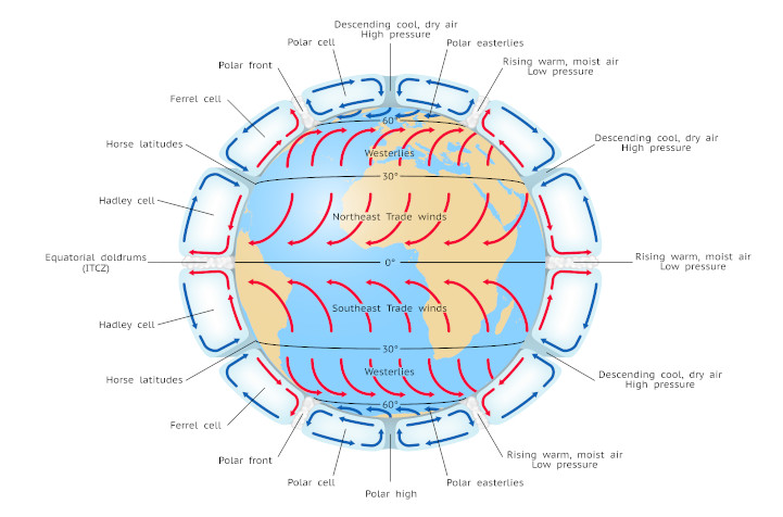
Another consequence of the Coriolis force is the deviation of the winds at the surface. The deviation of this winds in the Hadley cell form the persistent trade winds. In the Northern hemisphere, these winds flow from the tropic of the Cancer (60°N latitude) to the equator and from the tropic of the Capricorn (60°S latitude) to the equator in the southern hemisphere. These are deviated to the west to form northeast trade winds in the northern hemisphere and southeast trade winds in the southern Hemisphere.
The surface winds in the Ferrel cells flow from south to north (from the tropic of Cancer to the Arctic circle) in the northern hemisphere and from north to south (from the tropic of Capricorn to the Antarctic circle) in the southern hemisphere. These winds are deviated to the east. They form the southwest westerlies in the northern hemisphere and the northwest westerlies in the southern hemisphere.
The same happens in the Polar cells. The winds flow from the poles to the polar fronts and they are deviated to the West in both hemispheres, to form the polar easterlies.
Intertropical convergence zone (ITCZ)
The intertropical convergence zone is the region where the northeast trade winds from the northern hemisphere and the southeast trade winds from the southern hemisphere converge and rise to the troposphere. This zone encircle the earth and it is located near the equator.
Seasonal change in the atmospheric circulation and precipitation
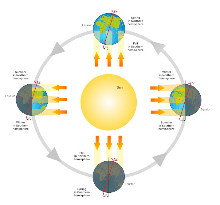
Because of the earth inclination and the rotation around the sun, the solar radiation is not the same at a point all the year. That is why we have season’s and that they are not the same between the northern hemisphere and the southern hemisphere. These seasons also affect the position of the different cells.
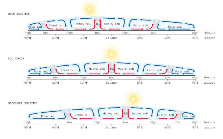
When it is summer in the northern hemisphere, the cells and the intertropical convergence zone move a few degrees to the north. On the opposite, in December the cells and also the intertropical convergence zone move to the south.
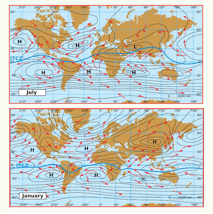
This leads to big local change in some area of the earth like the monsoon in India. In the winter the intertropical convergence zone is clearly defined and located in the Indian ocean, which lead to northeast continental winds. In the summer, the intertropical convergence zone is less defined and located above the continent and it brings southwest winds filled with rain.
The atmospheric circulation cells and climatic zones
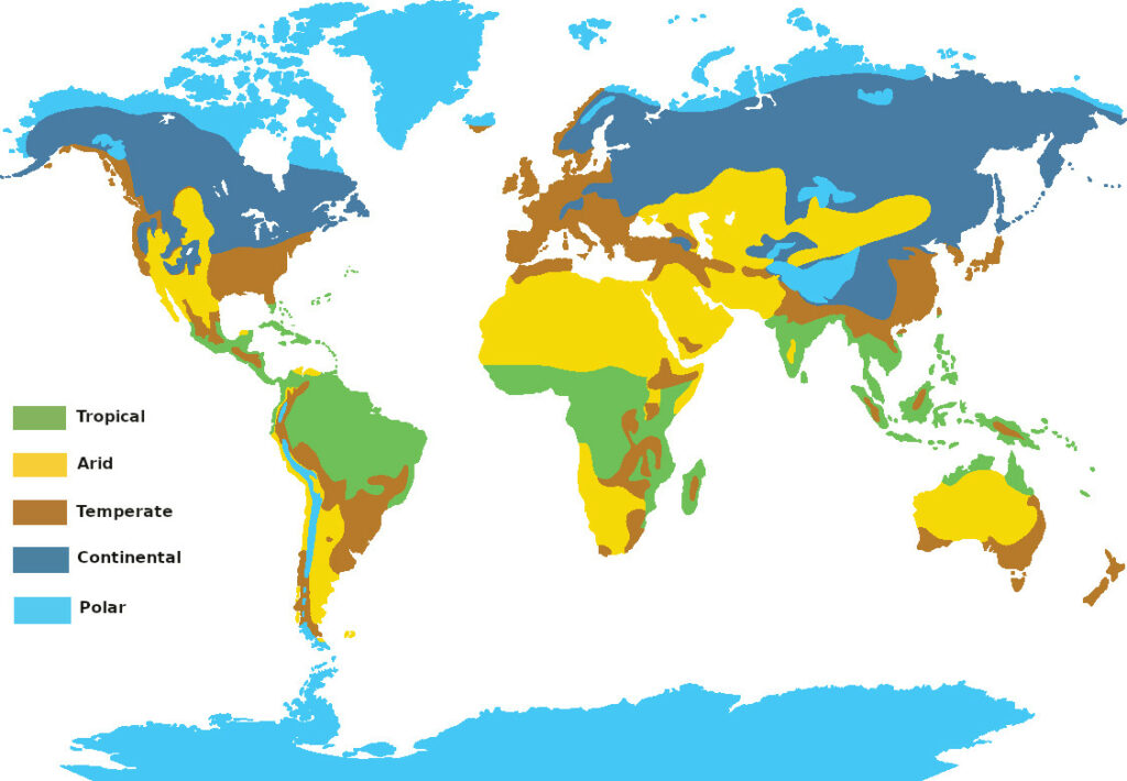
As explained previously, the different cells have an influence on the weather by defining semi permanent high and low pressure zone. And so the cells define the location of the different climatic zones of the earth.
Because of these cells, we have regions of semi permanent high and low pressure areas. At location of low pressure system, there is much more rainfall. On the opposite, high pressure areas give clear skies and so by consequence little rainfall, which leads to desert (cold and hot deserts).
That is why the largest areas of rainforest are located around the equator, because of the high solar radiation and the intertropical convergence zone that have as consequence daily afternoon rain, with a hot and wet atmosphere.
Arid climates, and so deserts, are located at the upper limit of the Hadley cells where dry air descends from the tropopause.
Polar regions are of course located at the pole and they are the consequence of the low solar radiation at the pole.
Foehn winds
Explore the fascinating world of Foehn winds, a captivating meteorological phenomenon that unfolds when prevailing winds encounter mountain ranges. These winds, also known as Föhn winds, create a unique climatic impact, resulting in dry and warm down-slope winds on the lee side of the mountains. Uncover the origins of the term “Foehn” from Swiss German and Latin influences, and delve into the intricate processes behind their formation. Discover how Foehn winds can influence precipitation, temperature, and cloud formations on the upwind slopes, while bringing warm, arid conditions on the downwind side. Journey through the diverse consequences of Foehn winds, from transforming landscapes and fostering deserts to their role in forest fires and sudden snowmelt. Join us as we unravel the intricacies of this meteorological marvel and uncover its intriguing effects on both nature and human well-being.
Table of contents
- Definition
- Where does the word Foehn come from?
- How do foehn winds form?
- Consequences of Foehn wind?
- Where are Foehn winds found?
- Foehn winds in California – Oregon and desert
- Foehn and Chinook winds?
- Foehn wind and other names?
- Foehn wind health effects
Definition
Foehn winds (also spelled Föhn winds) are meteorological phenomenon that happens when prevailing wind meets a mountain range. The result of this interaction is a dry and warm down-slope wind on the downwind side of the mountain range.
Where does the word Foehn come from?
The name Foehn come from the Swiss German Föhn which come from the Latin favōnius, a mild west wind. After it was adopted by the German Alpine dialects and designated a strong, dry and warm wind of the German Alps. This wind is where the phenomenon was first studied.
How do foehn winds form?

When the wind meets a mountain more or less perpendicularly, it follows the relief and rises. The atmospheric pressure decreases with the altitude and as a result the temperature of the air decreases by adiabatic expansion following the dry adiabatic lapse rate.
If the humidity is high enough at the beginning, since colder air can hold less water vapor, moisture will condense on the altitude point where saturation is reached (condensation level). So cloud will form and precipitation as rain and/or snow will occurs on the mountain’s upwind slopes.
The change of state from vapor to liquid water heats the air and partially counter the cooling of the air while it rises. Indeed, solar radiation, which provided heat and allowed the water to evaporate at ground level, is returned to the air by latent heat. The rate of decrease in the temperature of the air parcel will therefore be from this moment according to the saturated adiabatic lapse rate, as long as there is steam to condense. The rate of temperature variation for the dry air (dry adiabatic lapse rate) is around 10°C /km (around 5.5 °F per 1,000 ft) and of around 6°C / km (around 3.3°F per 1,000 ft) for saturated air (moist adiabatic lapse rate).
The Foehn effect don’t always produce rain, snow or even thick clouds on the upwind side. When there is no precipitation on the upwind side, and that if any clouds they have evaporated, then the temperature between the 2 sides of the mountain range are the same for the same altitude.
Consequences of Foehn wind?
They can be responsible for a difference of climate between each side of the mountain range. Indeed, when the upwind side is affected by rain and clouds, the down slope is affected by a dry and warm wind. This can be benefit, for example for vineyards, but this can also lead to desert on the down slope side of the mountain range. It can also be problematic for forest fire like it is the case in California.
Because of the strong wind, it can also create damage on the buildings and infrastructure.
Finally, the Foehn wind is also responsible for the sudden smelting of snow in regions where they are active.
Where are Foehn winds found?
These winds are found everywhere in the world where the prevailing wind meets a mountain range more or less perpendicularly. This phenomenon is global but, because the general circulation of the wind is along the parallels, it can be found at every mountain range oriented North – South.
Foehn winds in California – Oregon and desert

Like explain in a previous chapter, Foehn winds can be responsible for desertification. One example of this is the Sequoias and the Petrified forest on the United States west coast.
Until the Eocene the Rocky mountains and the Sierra Nevada mountain ranges were not so high and the Foehn had no effect on the lee (downwind side) because the air parcel didn’t go high enough to cross the condensation level. So the air parcel was following the dry adiabatic lapse rate on both sides of the mountain range and the vegetation was luxurious on both sides.
Then started the uplift of the Rocky mountains and the Sierra Nevada mountains. As a result the mountain range crosses the condensation level, and the upwind side began to be under clouds and precipitation condition. Because of this lose of water, the dry adiabatic lapse rate is reached more early on the downwind side. As a result the temperature on the lee is higher for the same altitude on the upwind side.
Like explain in the previous chapter the general circulation of the wind is along the parallels and so we can find the same type of desert on mountain range oriented North – South.

We have, for example, the Norwester (local Foehn wind name) in New Zealand that cause desert condition in the Marlborough region.

Another example of this is the Zonda (local name for the Foehn wind) in Chili and Argentina.
Foehn and Chinook winds?
Chinook winds are a local name for Foehn winds and it is used for the winds on the east sides of the Rocky Mountains in North America.
Foehn wind and other names?

We saw in the previous chapter that Chinook winds are a local name for Foehn winds, but there are other local names for this type of wind. Here is a list of some of them:
| Continent | Name | Location |
|---|---|---|
| Africa | Berg wind | South Africa |
| Asia | Loo | Indo-Gangetic Plain |
| Warm Braw | Schouten Islands north of West Papua, Indonesia | |
| Europe | Foehn | Alps |
| Fogony | Catalan Pyrenees | |
| Halny | Carpathian Mountains | |
| Helm | Cumbria, England | |
| North America | Chinook | East of the Rocky Mountains in Canada and the United States |
| Santa Ana | Southern California | |
| Oceania | The Norwester | East coast of New Zealand |
| Sout America | Puelche | Eastern wind that occurs in south-central Chile |
| Zonda | Eastern slope of the Andes in Argentina |
Foehn wind health effects
Following local believing, Foehn wind is linked with increased mental illness and states like aggressiveness, depression, suicide, anxiety, headaches, psychosis, …
Some modern studies are studying these believing and have shown an increase in suicides and accidents during episodes of Foehn.
Types of clouds and their characteristics
Clouds are in meteorology visible masses made of a big quantity of liquid droplets and /or frozen crystals suspended in the atmosphere. These clouds are formed by very small droplets of water and / or ice crystals (2 to 200 microns in diameter) obtained by the condensation of water vapor from the atmosphere around tiny particles (dusts, aerosols, …) called condensation nuclei.
The aspect of a cloud is characterized by its form, texture, opacity and colors. These parameters vary in function of the constituent of the cloud and the atmospheric conditions.
Table of contents
- How are clouds classified
- The 10 basic cloud types (genera)
- The 14 species of clouds
- The 9 varieties of clouds
How are clouds classified
The international classification uses the families, genera, species and varieties. This is similar to the classifications use for plants and animals and like these classifications, Latin names are used.
The nomenclature is based on 4 Latin names depending on the characteristics of the cloud.
| Names | Characteristics |
|---|---|
| Cumulus | rounded form |
| Cirrus | fibrous form |
| Stratus | layer without a specific form |
| Nimbus | accompanied by rain |
These names can be associated to define the different clouds of the classification.
In total the World Meteorological organization recognized currently 10 genera that are group in 4 families. Theses families correspond to 3 different altitudes intervals of the troposphere and 1 family for the clouds with high vertical development across the 3 different layers.
The 10 basic cloud types (genera)

| Family | Genera (name and symbol) |
|---|---|
| High clouds (ice) polar regions: 3 km to 8 km (10,000 to 25,000 ft)temperate regions: 5 km to 13 km (16,500 ft to 40,000 ft)tropical regions: 6 km to 18 km (20,000 ft to 60,000 ft) | Cirrus (Ci) |
| Cirrocumulus (Cc) | |
| Cirrostratus (Cs) | |
| Middle level clouds (liquid water / ice) polar regions: ~2 km to 5 km (6,500 ft to 16,500 ft)temperate regions: ~2 km to 9km (6,500 ft to 30,000ft)tropical regions: ~2 km to 12 km (6,500 ft to 40,000 ft) | Altocumulus |
| Altostratus (As) | |
| Nimbostratus (Ns) | |
| Low clouds 0 km to 2 km (0 ft to 6,500 ft) | Stratocumulus (Sc) |
| Stratus (St) | |
| Towering vertical polar regions: 0.5 km to 8km (1,650 ft to 25,000 ft)temperate regions: 0.5 km to 13 km (1,650 ft to 40,000 ft)tropical regions: 0.5 km to 18 km (1,650 ft to 60,000 ft) | Cumulus (Cu) |
| Cumulonimbus (Cb) |
Cirrus (Ci)

These are fibrous wisps of delicate white ice crystal clouds. They can be found in large fields or in narrow white bands. Sightly opaque, sunlight can pass through it. These clouds are pink or red after the sunset. These clouds don’t produce precipitation.
Cirrostratus (Cs)

These clouds are made of ice crystal and it forms a translucent whitish veil completely or partially covering the sky. These clouds are often accompanied by a halo phenomenon. This type of cloud also don’t produce precipitation, but it announces the arrival of a depression.
Cirrocumulus (Cc)

These clouds are rarely observed. They are shaped like a cotton flower and very small. They are composed of ice crystals or supercooled water droplets. These clouds are non-precipitating, but they can indicate the arrival of a front.
Altostratus (As)

These clouds are stratifom and they are present in layers in which the limits are difficult to define. They form a broad gray, slightly streaked or fibrous layer. They let light diffuse without a visible shadow on the ground. They have a thickness of 500 m to 3 000 m (1,650 ft to 10,000 ft). They are composed of water droplets, but it may be mixed with ice crystals at higher altitudes. Widespread opaque altostratus can produce light continuous or intermittent precipitation (rain or snow). These clouds are relative to a stable air.
Altocumulus (Ac)

These clouds are in the form of lamellae, pebbles, rolls with a sometimes partially fibrous or fuzzy appearance. They may or may not be welded. They are white and / or gray and they appear as a bank, in a sheet or in a layer. These clouds usually have their own shadow, which helps distinguish them from cirrocumulus clouds.
Stratus (St)

These clouds are characteristic grayish in color and have a fairly uniform appearance. They are sometimes made up of separate elements with a jagged appearance. They are often accompanied by a hazy atmosphere. They are also likely to give off drizzle (precipitation of very fine droplets of water or granulated snow (diameter less than one millimeter)). This type of cloud can result from nighttime cooling, the influx of humid air from a lake, sea or ocean, evaporation above a body of water or after heavy rain.
Stratocumulus (Sc)

This type of cloud appears as a large, dark, rounded mass. Individually, each cloud is bigger than an altocumulus cloud. They are usually present in groups, lines or waves. This type of cloud has a convective origin, but the vertical extension is immediately limited by the stability of the upper layer.
Cumulus (Cu)

This type of cloud is loose, normally dense, and budding in appearance (cauliflower-shaped) with a small vertical extension. This type of cloud occurs during convection following an adiabatic expansion. They can form in many types of situation, but often following the passage of a disturbance (the cold front moves away and the sun becomes visible again, which causes the ground to warm).
Cumulonimbus (Cb)

This type of cloud is dense with a very high vertical extension (the highest). It is of convective origin. The top has the shape of an anvil. This cloud is the source of thunderstorms and it generally develops as a cold front approaches.
Nimbostratus (Ns)

This cloud is stratiform with a significant vertical extension. It is often made up of several layered layers without a defined shape and dark gray in color. It also completely hides the sun. It produces low to moderate precipitation, but over large areas.
The 14 species of clouds
The 10 genera of clouds are the top classification, but most of the genera are subdivided into species due to the particularity in shape. A species can belong to more than one genera of cloud. One genera can have more than one species and some genera have no species. The species are mutually exclusive, in other word a cloud can be assigned to only one species.
| Species | Description | Genera |
|---|---|---|
| Fibratus | Detached clouds or a fine veil consisting of almost straight or more or less irregularly curved filaments and they do not end in hooks or tufts. | Cirrus and cirrostratus |
| Uncinus | Cirrus usually comma-shaped terminating in its upper part in a hook or tuft and the upper end of which is not in the form of a rounded protuberance. | Cirrus |
| Spissatus | Cirrus clouds thick enough to be gray when viewed near the sun. | Cirrus |
| Castellanus | Clouds which present in their upper part protuberances in the form of towers and which give them a crenellated appearance. The towers come from the same base and they are arranged in a line. | Cirrus, cirrocumulus, altocumulus and stratocumulus |
| Flocus | Each cloud is a tuft of cumuliform appearance, the base of which is more or less jagged and which is often accompanied by virga (observable streak or shaft of precipitation falling from a cloud that evaporates or sublimates before reaching the ground). | Cirrus, cirrocumulus and altocumulus |
| Stratiformis | Clouds that extend in a large sheet or horizontal layer. | Stratocumulus, altocumulus and sometimes cirrocumulus |
| Nebulosus | Clouds in the form of a veil or layer, with no distinct detail. | Stratus and cirrostratus |
| Lenticularis | Lentil or almond shaped clouds, often elongated and with a well-defined perimeter shown by an iridescence. | Stratocumulus, altocumulus and cirrocumulus |
| Fractus | Clouds in the form of irregular rags with a distinctly jagged appearance. | Stratus and cumulus |
| Humilis | Cumulus of weak vertical extension. | Cumulus |
| Mediocris | Cumulus of average vertical extension and whose top shows small protrusions | Cumulus |
| Congestus | Cumulus of great vertical extension, the upper part of which resembles a cauliflower | Cumulus |
| Calvus | Cumulonimbus whose summit protuberances begins to lose their cumuliform appearance, but in which we can’t distinguish from cirriform parts. | Cumulonimbus |
| Capillatus | Cumulonimbus characterized by the presence at its summit of cirriform parts fibrous or striated, anvil-shaped, of plume or a large mass of more or less messy hair. It is often accompanied by a downpour or a thunderstorm. | Cumulonimbus |
The 9 varieties of clouds
We have finally the classification following to the 9 varieties of clouds. The varieties are function of the arrangements of the elements and the degree of transparency of the genera. The varieties aren’t mutually exclusive, in other word a cloud can be of different varieties. Only the varieties translucidus and opacus are mutually exclusive. It is important to note that clouds don’t have necessary to belong to one or several varieties.
| Varieties | Description |
|---|---|
| Intortus | Cirrus with irregularly curved and often twisted filaments. |
| Vertebratus | Mainly cirrus clouds arranged in the shape of vertebrae, ribs or having the appearance of the skeleton of a fish. |
| Undulatus | Clouds in the shape of waves and whose elements are sometimes separated, sometimes juxtaposed. |
| Radiatus | Clouds in parallel bands that seem to converge towards a point on the horizon |
| Lacunosus | Layer or cluster in which we find circular orifices equally distributed or clusters resembling a honeycomb. |
| Duplicatus | Multilayer (at different heights) of the same type of cloud. |
| Translucidus | Layer or cluster of fairly large horizontal dimension that allows to see the sun or the moon |
| Perlucidus | Quite large layer or cluster with distinct gaps, but sometimes rather small, and which let see the sun, the moon, the sky or other clouds. |
| Opacus | Large layer or cluster thick enough to mask the sun or the moon. |
Polders
Polders are land reclaimed from water by population and it is most specifically associated with the Netherlands. Indeed, they have acquired through the century a very broad knowledge in this domain. Before we start to show how important they are for the Netherlands, we need to understand what they are and how they are made.
Table of contents
- What is a polder?
- How are polders made?
- Where are polders found?
- Polders in Bangladesh
- Polders in the Netherlands
- Why are Polders important to the Netherlands?
- Polders and dikes in the Netherlands
- The Delta Works
What is a polder?
A polder is an artificial tract of land reclaimed from water from marshes, estuaries, lakes or coastal areas. Most often the level of the tract of land is lower than that of the sea.
How are polders made?
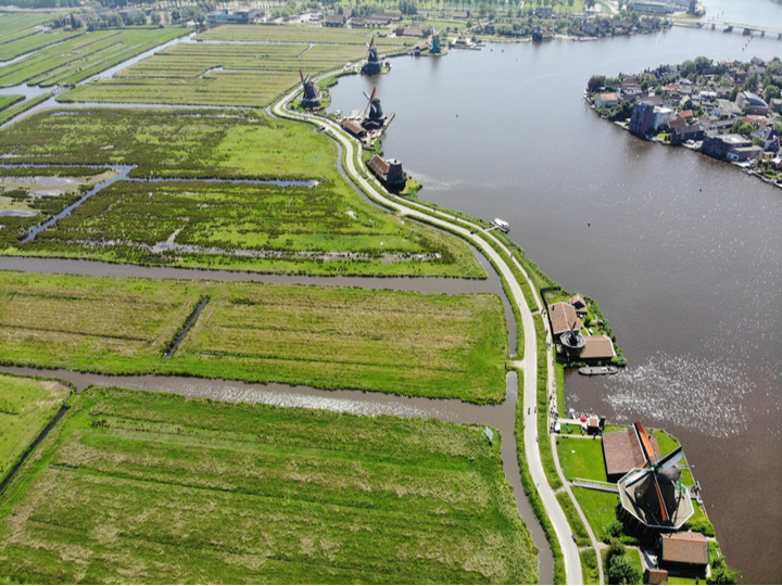
The surface to be developed is first surrounded by dikes. The water trapped between the dikes is then pumped. This was in the past operated by windmills equipped with a worm screw to raise the water to the sea, river or a channel. When this channel is also lower than the sea the water of the channel is also pumped into the sea with a windmill equipped with a worm screw. At the 19th century, these windmills were replaced by steam machines and by electrical and diesel motors in the 20th century.
The pumping of the water is not sufficient. To make the ground more dry, some plants, like reeds, are planted to dry up the ground.
To avoid the flooding of the polders by rain, a network of channels is built in the polders to drain all this water.
After the polder is built, the pump continues to work daily.
Where are polders found?
Polders are associate with Belgium and more notably with the Nederlands because a a substantial part of their area has been reclaimed from the sea over the centuries. But they are also found in Bangladesh, Canada, China, Denmark, Finland, France, Germany, Guyana, India, Ireland, Italy, Lithuania, Poland, Slovenia, South Korea, Spain, United Kingdom and United States.
Polders in Bangladesh
Bangladesh has 123 polders that are distributed along the sea (49 polders) and along the numerous distributaries of the Ganges – Brahmaputra – Meghna Rivers delta. These polders are recently built (in the 1960s) to protect the coast from tidal flooding and to reduce the salinity incursion for the agriculture.
Polders in the Netherlands
The Netherlands is frequently associated with polders because of their use across the centuries and their knowledge they have developed in this domain.
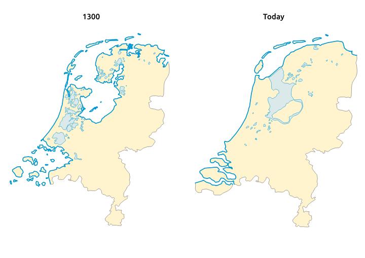
The Netherlands has started their conquest on land since the 13th century. 3 big periods of works can be distinguished. Between the 13th century and the 18th century, they have worked in the south and north of the country. Between the 18th century and all the 19th century the works where concentrated on the west of the country. And finally in the 21st century, they decided to build a full new province in the Zuiderzee, the Flevoland.
Why are polders important to the Netherlands?
The area of the Netherlands is 41 526 km², with 7 150 km² of polders, which represent 17% of the territories. In the beginning with the windmills, the soils were not dry enough for the agriculture and the polders where only use for breeding. After 1850 and the use of new technologies they managed to have the groundwater always at more than 1 m below the ground level of the polder which have allowed agriculture and the building of houses. Nowadays 60 % of the population the Netherlands lives on polders.
Polders and dikes in the Netherlands
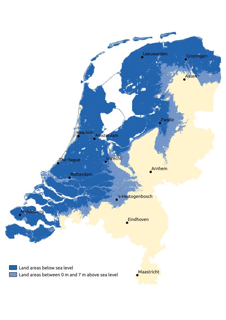
With this conquest over the sea a total of around 25% of the Netherlands are below the water level with a maximum of -6.76 m below the sea level, which is maximum for Europe. To protect these lands there are sand dunes all along the coastline. But these are not sufficient and dikes had to be built. Without these dikes, in times of high tide water would invade the land.
Another danger comes also from the rivers that have difficulties to flow down to the seashore because of the flatness of the Netherlands. If there where no dikes around these rivers, the water of the rivers will also invade the land.
Without all these infrastructures, more than the half of the country would be subject to flooding.
The Delta Works
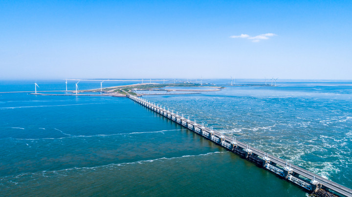
The Delta is a region of the south of the Netherlands, where the Rhine, Meuse and Scheldt flows into the North Sea. For a long period this region was very vulnerable because the sea could flood into the lands by using these 3 rivers like it has happened in 1953 and cause the death of 1800 persons. To avoid this to happen again, all the dikes were heightened to resist to a tide of 5m. But there was still 700 km of dikes to control. The government decided in the 1950s to close the inlets by building dams. These have bring to 25 km the dikes facing the sea, which is more easy to control.
Volcanoes
A volcano is a geological structure that results from the rise of magma and then from the eruption of materials (gas and lava) from this magma, on the surface of the earth’s crust (or another planet). It can be aerial or underwater. Because it is linked with a rise of magma most of them are directly linked with tectonic plates and this explain the localisation of volcanoes on the world map.
Table of contents
- Structure of volcanoes
- Type of volcanoes
- Tectonic plates and volcanoes world map
- The Pacific Ring of Fire
- Top 10 biggest volcanoes in the world by height
- Recommended books
Structure of volcanoes
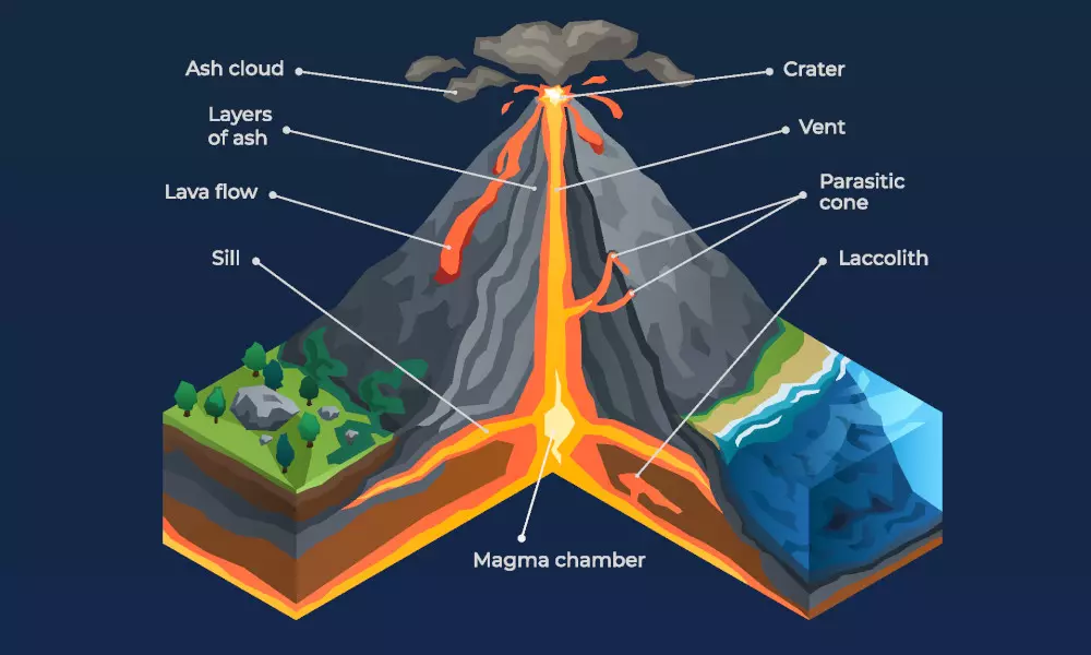
A volcano is made up of different structures that are generally found in each of them:
- Magma chamber: filled by magma coming from the mantle and playing the role of reservoir and the place of differentiation of the magma. When it empties following an eruption, the volcano can collapse and give birth to a caldera. The magma chambers are between 10 and 50 km deep in the lithosphere.
- Vent: pipe that conduct magma from the chamber to the surface.
- Crater (or a Caldera): place of the opening of the vent on the surface.
- Secondary volcanic vents: starting from the magmatic chamber or the main vent and generally leading to the sides of the volcano, sometimes at its base. Further, they can give rise to small parasitic cones.
Type of volcanoes
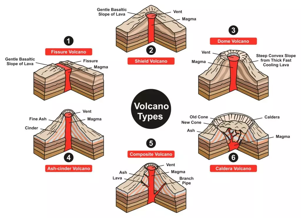
- Fissure volcano: formed by a linear opening in the continental or oceanic crust through which escapes fluid lava. We have, for example the oceanic ridge for this type of volcanoes.
- Shield volcano: the diameter is much greater than its height due to the fluidity of the lavas which can travel for kilometers before stopping. For example, the Mauna Loa in Hawaii is a shield volcano.
- Dome volcano: large volcanic dome formed by the accumulation of slow eruptions of highly viscous lava. The Puy de Dôme is an example of this kind of volcano.
- Volcanic cones (or cinder cones): it results from eruptions of mostly small pieces of scoria and pyroclastics (both resemble cinders, hence the name of this volcano type) that build up around the vent.
- Stratovolcanoes (composite volcanoes): the diameter is more balanced compared to its height due to the greater viscosity of the lavas; these are volcanoes with explosive eruptions. The conical mountain is composed of lava flows and other ejecta in alternate layers. For instance, the Mount Fuji in Japan is an example of this type of volcano.
- Caldera volcano: large depression due to the collapse of rocks above a magma chamber. The Yellowstone caldera is an example of the caldera.
- Maar: low-relief volcanic crater caused by a phreatomagmatic eruption ( explosion that occurs when groundwater comes into contact with hot lava or magma). A maar characteristically fills with water to form a relatively shallow crater lake which may also be called a maar.
Tectonic plates and volcanoes world map
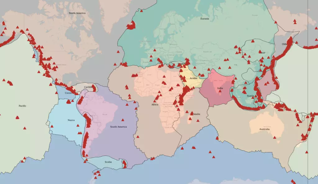
If you look to the volcanoes world map, you can see that most of them are linked to tectonic plates boundaries. Firstly, we will present the 2 types of volcanoes linked to the tectonic plates. Then we will see the last type of volcanoes which are not linked to the plate tectonics.
Divergent plate boundaries
At the ridge, the separation of two tectonic plates thins the lithosphere, causing a rise in mantle rocks. These, already very hot, start to melt partially due to decompression. This gives magma which infiltrates through normal faults. Between the two edges of the rift, traces of volcanic activity such as pillow lava (formed by the emission of fluid lava in cold water). Thus, these volcanic rocks constitute a part of the oceanic crust.
In the continental rifts, the same process occurs, except that the lava does not flow underwater and does not give pillow lava.
Convergent plate boundaries
When two tectonic plates overlap, the oceanic lithosphere, sliding under the other oceanic or continental lithosphere, plunges into the mantle and undergoes mineralogical transformations. The water contained in the plunging lithosphere then escapes and hydrates the mantle, causing its partial melting by lowering its melting point. So, this magma rises and crosses the overlapping lithosphere, creating volcanoes.
If the overlapping lithosphere is oceanic, an island volcanic arc will form, the volcanoes giving rise to islands. This is the case for the Aleutians and Japan.
If the overlapping lithosphere is continental, the volcanoes will be located on the continent, generally in a cordillera. This is the case of the Andean volcanoes or the Cascade range. These volcanoes are generally gray, explosive and dangerous volcanoes. This is due to their viscous lava because it is rich in silica, which has difficulty flowing; moreover, the magmas which rise are rich in dissolved gases (water and carbon dioxide), the sudden release of which can form fiery clouds. The “Pacific Ring of Fire” is made up almost entirely of this type of volcano.
Hot spot
It sometimes happens that volcanoes are located far from any lithospheric plate boundary. They are generally interpreted as hot spot volcanoes. The hot spots are plumes of magma coming from the depths of the mantle and piercing the lithospheric plates.
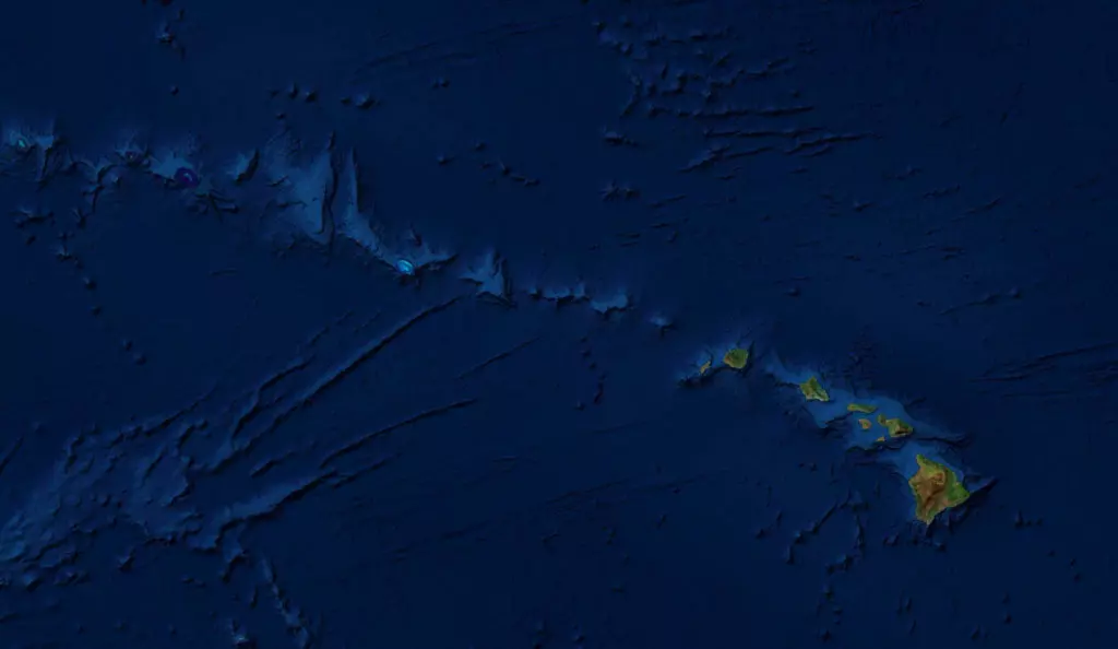
The hot spots being fixed, while the lithospheric plate moves on the mantle, volcanoes are created successively and align then, the most recent being the most active because at the base of the hot spot. When the hot spot emerges under an ocean, it will give birth to a series of aligned islands as is the case of the Hawaiian or Mascarene archipelago.
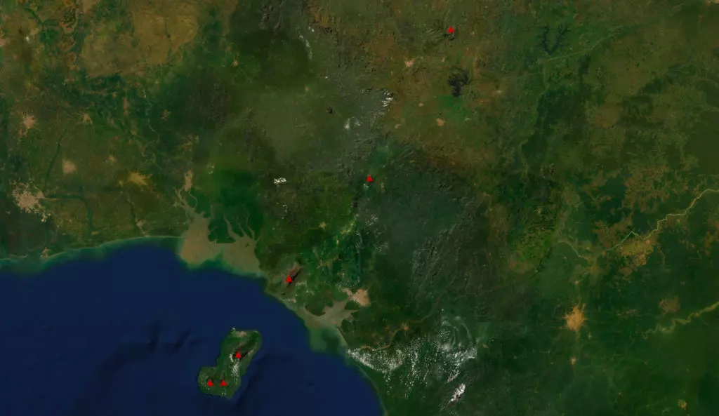
If the hot spot emerges under a continent, it will then give birth to a series of aligned volcanoes. This is the case of Mount Cameroon and its neighbors.
In exceptional cases, it happens that a hot spot opens out under a lithospheric plate boundary. In the case of Iceland, the effect of a hot spot combines with that of the mid-Atlantic ridge, thus giving rise to a huge stack of lava allowing the ridge to emerge. The Azores or Galápagos are other examples of hot spots opening out under a lithospheric plate boundary.
However, many intra-plate volcanoes do not occur on alignments to identify deep and permanent hot spots.
The Pacific Ring of Fire
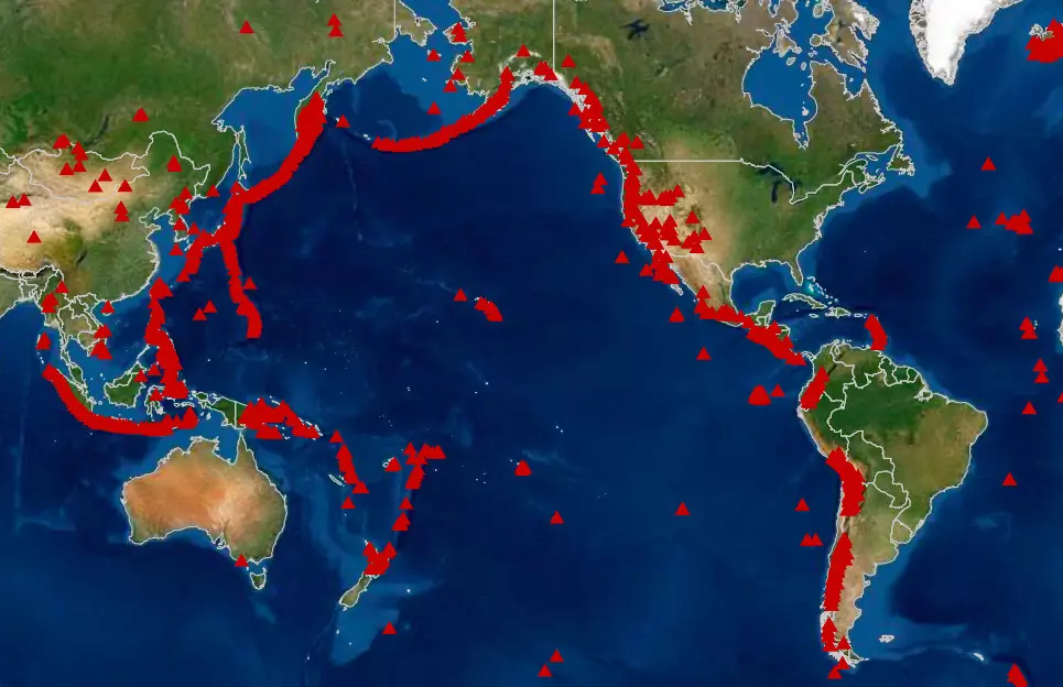
The Pacific Ring of Fire (also known as the Rim of Fire or the Circum-Pacific belt) designates the alignment of volcanoes that border the Pacific Ocean over most of its periphery, approximately 40,000 km (25,000 mi) .
This alignment of volcanoes, all located exclusively on the coasts or islands, coincides with a set of limits of tectonic plates and faults. These limits are also marked by the main ocean trenches on the planet.
Top 10 biggest volcanoes in the world by height
1. Mauna Kea, Hawaii
This volcano is 4,207 m above sea level, but with its part under water, it is 10,203 m (33,474 ft). It makes this volcano in total height even higher than the Mount Everest. This volcano is a hot spot in the pacific plate.
2. Mauna Loa
Secondly, we find another volcano of Hawaii, which is made of 5 volcanoes. This volcano is 9,170 m (30,085 ft) from the bottom of the sea level.
3. Haleakalā or East Maui Volcano
On the 3th place, we have another volcano of Hawaii. This volcano is 9,144 m (30,000 ft).
4. Teide
This volcano is located on the island of Tenerife. It has an altitude of 3,718 m (12,198 ft) above sea level. From the bottom of the sea level, it is 7,500 m (24,606 ft).
5. Piton des Neiges
It is the massive shield volcano on the Reunion. From the bottom of the ocean, it has a total elevation of 7,071 m (23,199 ft).
6. Ojos del Salado
This volcano is located in the Andes on the Argentina – Chile border. It is the highest active volcano in the world. It has an altitude of 6,893 m (22,615 ft).
7. Monte Pissis
This volcano is an extinct volcano located in Argentina and it has an elevation of 6,792 m (22,283 ft).
8. Nevado Tres Cruces
This volcano is also located in the Andes on the Argentina – Chile border. It has an elevation of 6,748 m (22,139 ft).
9. Llullaillaco
This volcano is also located on the border between Argentina and Chile. It has an elevation of 6,739 m (22,110 ft).
10. Tipas
Finally the last volcano of our list is also located in the Andes on the border between Argentina and Chile. It has an elevation of 6,670 m (21,880ft)
Time Zones
A time zone is a region of the globe that observes a uniform standard time for legal, commercial and social purposes. They tend to follow the boundaries of countries instead of strictly longitude, because it makes more sense for commercial and communication reasons to keep the same time. We will dive into more details in the time zone in this section. Our interactive world map of the time zone gives also the possibility to see the time in each time zone and the time in your time zone.
Table of contents
- Why do we have time zone
- History
- Greenwich Mean Time (GMT)
- Coordinated Universal Time (UTC)
- Time zones in the Polar regions
- International waters
- Daylight saving time (DST)
Why do we have time zone

The reason that we have time zones is directly linked by the shape of the earth. The spherical shape of the earth turns on its axis (poles) with a complete rotation in 1 day, so in other words 24 hours.
the earth is turning around the sun in around 365 days and 6h. During its turn around the sun, the earth rotates and different part of the Earth receives sunlight and the other part is in the dark, which give the day and night.
Without time zone, if we take midday (12h PM) in function of our location on the earth this time will be in the morning, midday, evening or at night.
Since always populations have lived in different time zones, but without being conscious of it or with a different organisation has it is today. The next chapter will take a look into the history. This will explain how we arrived to the actual time zone.
History
Before clocks
Before the the clock was invented, people were measuring time with different early measuring device like sundials and water clocks.
Discovering of the mechanical clocks
The mechanical clocks appear around the end of the 13th century. At that time, there was a very limited number of water and mechanical clocks. They were only frequent in monastery and cathedrals. At the beginning these clocks were only there to ring 24 times the bell (for the 24 hours).
Later the technical advances have allowed to display the 24 hours. In the beginning, it is the 24 hours that will move and then it will be fixed and only the clock hand for the hour will move. Further improvement will simplifying the 24 parts in 12 parts for readability. The clocks will become more little. In the 14th century, the church towers across Europe had clocks so that they were visible for everyone.
Across the 15th century, improvements and miniaturisation continues. In the 15th century we started to have the first table clocks and even the first watch with ringing clocks on costume of people at the end of the 15th century.
Greenwich Mean Time (GMT)
The Greenwich Mean Time (GMT) was established in 1675 when the Royal Observatory was built. It was an aid to mariners to determine longitude at sea, providing a standard reference time while each city in England kept a different local time. To calculate the longitude from the Greenwich meridian, British mariners kept at least one chronometer on GMT. The convention from the International Meridian Conference of 1884 set the Greenwich meridian as the longitude zero degrees.
The GMT start to become a standard time independent location because of this practice and the use of mariners from other nations of the lunar distances based on observations at Greenwich. Most time zones were based upon GMT, as an offset of a number of hours (and also half or quarter hours) ahead of GMT or behind GMT.
Railway time: the first standard time zone
With the development of transport and telecommunications, local solar time starts to become increasingly inconvenient, because clocks differed between places in function of the geographical longitude. The variation of time with the geographical longitudes is about 4 minutes by degree of longitude in the United Kingdom. For example, when it is solar noon in Bristol, it is about 10 minutes past solar noon in London.
The first adoption of a standard time zone was established in Great Britain on November 1840 using the GMT kept by portable chronometers. The first company to adopt the standard time was the Great Western Railway (GWR). This quickly became known as Railway Time.
Then around the 23 august 1852, the Royal Observatory of Greenwich emitted time signals for the first time by telegraph. By 1855, 98% of the Great Britain’s public clocks were using GMT, but it was still not Britain’s legal time until 2 August 1880. Clocks with 2 minutes hands was common at that period. One of the minute hand was for the local time and the other one for GMT.
The meridian of Rome and the first time zone world map
Quirico Filopanti, an Italian mathematician, proposed the first worldwide time zones in1858. That year, he published the idea in his book Miranda. In it, he proposed 24 time zone of 1 hour that he describe has longitudinal days. The first of his longitudinal day was centred on the meridian of Rome. He also proposed a universal time for Astronomy and telegraphy. His book didn’t have an impact at that time and it was not adopted worldwide.
The first country to adopt a standard time
The first country to adopt a standard time throughout all the colony was New Zealand in 1868. This standard was known as New Zealand Mean Time and was 11 hours 30 minutes ahead of GMT.
American Railways
Timekeeping on the US railroad in the middle of the 19th century was very confused. Each railroad was using its own standard time. This standard time was based on the local time of its headquarters or an important terminus. Companies use their own standard time to publish their railroad’s train schedules. Junctions with several railroads had a clock for each railroad and each one showing a different time. For example the Central station of Pittsburgh in Pennsylvania had 6 different hours.
Around 1863, Charles F. Dowd proposed a standard 1-hour time zones for the American railways. He didn’t publish anything at that time and it is only around 1869 that he consult the railroad officials. In 1870, he proposes 4 time zones with straight North-South separation. The first time zone was centered on Washington. In 1872, some changes were made and the first time zone was centered on the meridian 75° of Greenwich. Furthermore, geographic borders limited the time zones like for example the Appalachian Mountains. American Railroads companies never accepted the System of Dowd.
Instead, the US and Canadian railroad companies implemented the version proposed by Wiliam F. Allen, the chief editor of the Traveler’s Official Railway Guide. The border of the time zones in this system ran through stations and most of the time in important cities. For example, the border between the Eastern and the Central Time zones cross through Detroit, Buffalo, Pittsburgh, Atlanta and Charleston. The system was adopted on Sunday 18 November 1883, also called “the day of the 2 noons”. That day, each station changed the time to the standard time when the clock reached the noon.
Intercolonial, Eastern, Central, Mountain and Pacific are the 5 zones of this system. After one year, 95 % of the cities above 10 000 inhabitants (around 200 cities) had adopted the system. A big exception was the city of Detroit. Located in the middle of a time zone it holds local time until 1900.
The meridian of Greenwich for the time zone world map
In 1876, the Canadian Sandford Fleming proposed to generalize the concept of the American railroads time zone worldwide. First, he proposed a concept of a global 24 hour clock linked to any surface meridian. In 1879, he specifies that the universal day begins at the anti-meridian of Greenwich (180th meridian). He continued the promotion of his system on international conference. In October 1884, the International Meridian Conference didn’t adopt his time zone because they were not within its purview. But the conference did adopt a universal day of 24 hours beginning at Greenwich midnight. They also specified that this system shouldn’t interfere with the use of local or standard time where desirable.
In 1900, almost all inhabited places had adopted one or other standard time zone, but only a few of them used an hourly offset from GMT. It was more common to apply the time of a local astronomical observatory to the entire country without any reference to GMT. It took a few decades before GMT was generalized. In 1929, most major countries had adopted the standard GMT system. Nepal was the last country and adopted it in 1956.
Greenwich Mean Time (GMT)
The Greenwich Mean Time or GMT is the mean solar time at the Greenwich meridian. This meridian is the origin of the longitude and cross the Royal Observatory in Greenwich near London in the United Kingdom.
The time reference in the major part of the 20th century was the Greenwich Mean Time. Finally, the Coordinated Universal Time (UTC) replace it in 1972.
The need of another system is due to the fact the measure is inaccurate due to the uneven angular velocity of the earth, its elliptical orbit and its axial tilt.
GMT is still often used as a synonym for UTC. The 2 measures are close, but they are not totally the same because the GMT is based on the earth rotation and the UTC is based on the International Atomic Time.
Coordinated Universal Time (UTC)
The coordinated Universal Time or UTC is the measurements between the International Atomic Time (TAI) and the Universal Time (TU). The TAI is stable, but there is no connection with the earth rotation. The TU is connect with the earth rotation and so he variate a bit.
The name UTC is due to the division between French speakers (Temps Universel Coordonné – TUC) and English speakers (Coordinated Universal Time – CUT). UTC was a compromise between the 2.
Today, this system is use for the time zones around the world with positive and negative offsets from UTC. This offsets range from UTC-12:00 in west to UTC+14:00 in the east.
It is important to remark that Daylight saving time doesn’t change the UTC time. It is the local time that may change with summer time, but not the UTC time.
Time zones world map in the Polar regions
Science stations in the Arctic and Antarctic use generally the time zone of their supply base. So, the Amundsen-Scott station located in the South Pole uses the time zone of New Zealand. It means UTC+12 in the Austral winter and UTC+12 in the Austral summer.
A zone without scientific installation have no official time zone. Near the North Pole, it is possible to use UTC +- 0 by convention.
International waters
Boats in international waters generally change hours when they cross the meridians that limits a time zone like their definition at the origin. However, there is no fixed convention and boats use what is the most convenient for them.
Daylight saving time (DST)
The daylight saving time (United States and Canada) or summer time (United Kingdom, European Union, and some other country) is the practice to advance the clock of 1 hour for the warmer months of the year. More temperate regions use this system because the season light variation is higher. The interest is to delay the sunrise and sunset during this period. Another interest is the energy saving. Indeed, it allows to having day light until later in the day.
The transition between the normal time and the summer time depends on the countries. For Europe the period is between the last Sunday of march to the last Sunday of October. In North America it goes from 2nd Sunday of march to the first Sunday of November. The change happens between midnight and 4 h in function of the countries.
Earthquakes
An earthquake is the shaking of the surface of the Earth resulting from a sudden release of energy in the Earth’s lithosphere that creates seismic waves. This release of energy takes place by rupture along a fault, generally pre-existing. More rarely they are due to volcanic activity or of artificial origin (explosions for example).
Table of contents
- What causes earthquakes
- Tectonic earthquakes
- Earthquakes of volcanic origin
- Main features of an Earthquake
- Types of seismic waves
- Measuring of earthquakes (Magnitude)
- Frequency and effects
- Largest earthquakes since 1900
What causes Earthquakes
An earthquake is a more or less violent shaking of the ground which can have four origins:
- rupture of a fault or a segment of fault (tectonic earthquakes)
- intrusion and degassing of a magma (volcanic earthquakes)
- “Cracking” of ice caps echoing through the earth’s crust (polar earthquakes)
- explosion, cavity collapse (earthquakes of natural origin or due to human activity).
Tectonic earthquakes
Tectonic earthquakes are the result of movement along faults that suddenly release the stored elastic strain energy.
Most of the tectonic earthquakes takes place at the edges of the tectonics plates. Another part takes place along an existing or newly formed fragility plane.
Type of Earthquake faults
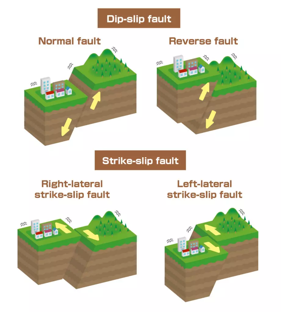
These faults are of three main types: normal, reverse and strike-slip.
Normal faults are dip-slip and so involve an vertical movement. In a normal fault, the block above the fault moves down relative to the block below the fault. Normal faults occur mainly in areas where the crust is being extended, like as in divergent boundaries. Earthquakes linked with normal faults have generally a magnitude less then 7. At the level of the mid-ocean ridges, earthquakes have superficial foci (0 to 10 kilometers), and correspond to 5% of the total seismic energy.
The reverse fault is the opposite of the normal fault, the block above the fault moves up relative to the block below the fault. Reverse faults occur in areas where the crust is being shortened like at convergent boundaries. These faults, particularly those along convergent plate boundaries are associated with the most powerful earthquakes. In subduction zones, earthquakes represent half of those that are destructive on Earth, and dissipate 75% of the earth’s seismic energy. It is the only place where we find deep earthquakes (from 300 to 645 km).
The Strike-slip fault is a steep structure where the 2 blocks move horizontally. Transform boundaries are example of strike-slip faults. These faults, particularly in transform boundaries, can produce major earthquakes, up to a magnitude of 8. at the level of large strike-slip faults, earthquakes occur with centers of intermediate depth (from 0 to 20 kilometers on average) which correspond to 15% of the energy.
Release of the accumulated energy does not usually happen in a single time, and it may take several readjustments before regaining a stable configuration. Thus, aftershocks are observed following the main shock of an earthquake, of decreasing amplitude, and over a period ranging from a few minutes to more than a year.
Intraplate Earthquake
Intraplate earthquakes are earthquake that occurs within the tectonic plate, in contrast with earthquakes at the boundaries of tectonic plates.
These earthquakes are rare compared to the earthquakes on the boundaries of the tectonic plates.
All tectonic plates have internal stress field caused by their interactions with neighboring plates, sedimentary loading or unloading (for example by deglaciation). The accumulation of these stresses may be release along existing fault plane and having has consequence intraplate earthquakes.
Earthquakes of volcanic origin
Earthquakes of volcanic origin result from the accumulation of magma in the magma chamber of a volcano. The seismographs then record a multitude of microseisms due to ruptures in the compressed rocks or to the degassing of the magma. The gradual rise of hypocenters (linked to the rise of magma) is an indication that the volcano is waking up and that an eruption is imminent.
Main features of an Earthquake
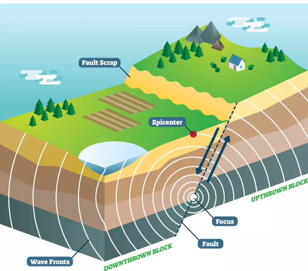
The hypocenter (or focus) is the point of initial rupture. It can be located between the surface and 670 km (420 mi), which is the limit between the upper and lower mantle.
The epicenter is the point on the surface of the earth directly above the hypocenter.
Types of seismic waves
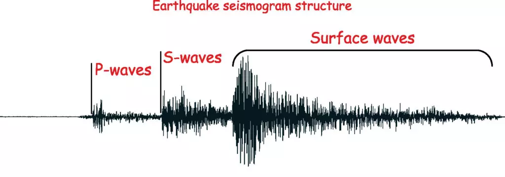
At the time of the sudden release of the constraints of the earth’s crust (earthquake), two main categories of waves can be generated. These are body waves that propagate inside the Earth and surface waves that propagate along the Earth’s surface.
Body waves
The body waves are divided in 2 types of wave as a result of 2 types of particle motion:
P-waves (Primary waves) or compression waves
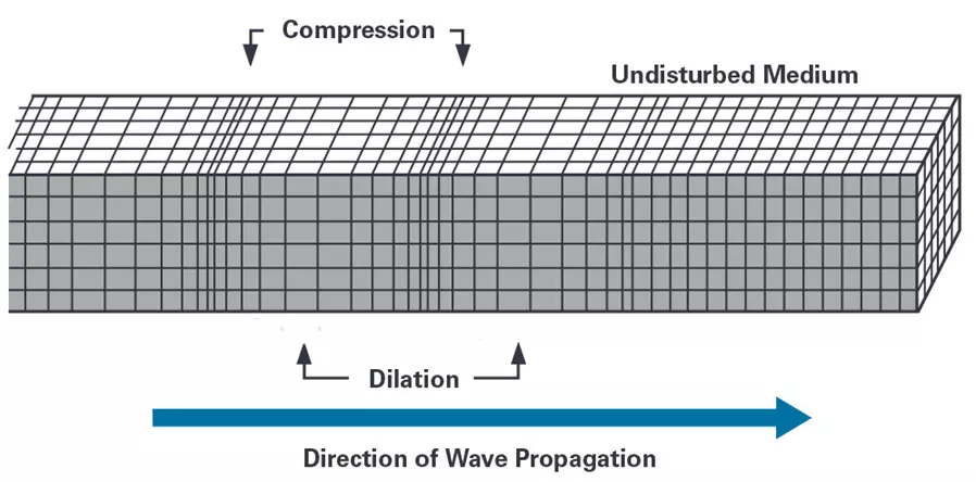
The ground is moved by successive expansion and compression, parallel to the direction of wave propagation. P waves are the fastest (6 km / s near the surface). So these are the waves recorded first on a seismogram and these wave can travel in any type of material (including fluids).
S-waves (Secondary waves) or shear waves
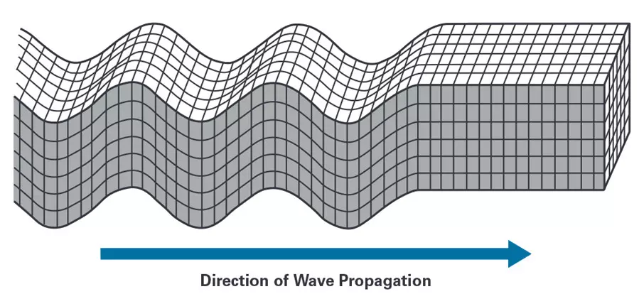
The vibrations are perpendicular to the direction of propagation of the wave. Slower than P waves, they appear second on seismograms. The S-wave are around 60% more slowly then the P-wave in any given material. The S-waves are not able to travel in liquid. Their absence in the earth’s outer core and so it suggests a liquid state.

Surface waves
Seismic surface waves propagate along the Earth’s surface. They are more slowly than seismic body waves (P-waves and S-waves). They can reach an amplitude of several centimeters in big earthquakes and they are usually the waves responsible of the destructive effects of earthquakes.
We can distinguished 2 type of surface waves:
Rayleigh waves
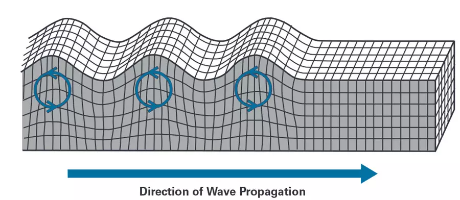
These waves includes both longitudinal and transerve motions that decrease exponentially in amplitude as distance from the surface increases. They are generated by the interaction of P-waves and S-waves. They are more slowly than P-wave and S-wave (around 90% of the velocity of S-waves)
Love waves
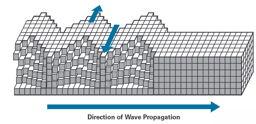
These waves are horizontally polarized surface waves. They are the result of the interference between many S-waves. They are slower than P- and S- waves, but faster than the Rayleigh waves.
Measuring of earthquakes (Magnitude)
The magnitude is in seismology the logarithmic representation of the seismic moment, which is itself a measure of the energy released by an earthquake.
The more energy the earthquake has released, the higher the magnitude: an increase in magnitude of 1 corresponds to a 30 times increase in energy and a 10 times increase in the amplitude of movement.
The media often use the term of Richter scale or open Richter scale, but these terms are not correct. Indead, the Richter scale is a local scale especially adapted to the Califonian earthquakes. The magnitudes usually cited nowadays are in fact moment magnitudes.
The following types of magnitudes are defined:
- Richter Scale or the local magnitude scale (ML or ML)
- mB scale that are calculated from body-wave
- MS scale that are calculated from surface waves.
- The moment magnitude scale (Mw) is based o an earthquake’s seismic moment.
Seismic magnitude scale and intensity scales are two different measures. Intensity is a measure of the damage caused by an earthquake. The intensity can have different values for the same earthquakes. Relationships between the maximum felt intensity and the magnitude exist but they are very dependent on the local geological context. These relationships are usually used to find the magnitude of historical earthquakes.
Frequency and effects
| Description | Moment magnitude scale | Effects | Global average frequency |
|---|---|---|---|
| Micro | < 1.9 | Micro earthquake, not felt. | 8,000 / day |
| Very minor | 2.0 – 2.9 | Usually not felt. | 1,000 / day |
| Minor | 3.0 – 3.9 | Often felt but without causing damage. | 50,000 / year |
| Small | 4.0 – 4.9 | Noticeable shaking of objects inside houses, clashing noises. The damage remains very light. | 6,000 / year |
| Moderate | 5.0 – 5.9 | Can cause significant damage to poorly designed buildings in restricted areas. No damage to well-constructed buildings. | 800 / year |
| Strong | 6.0 – 6.9 | Can cause serious damage for several tens of kilometers. Only adapted buildings resist near the center. | 120 / year |
| Very Strong | 7.0 – 7.9 | Can cause severe damage over large areas; all buildings are affected near the center. | 18 / year |
| Major | 8.0 – 8.9 | Can cause very severe damage in areas hundreds of kilometers around. Major damage to all buildings, including tens of kilometers from the center. | 1 / year |
| Near total destruction | 9.0 and more | Devastates areas for kilometers of miles around. Damage over 1,000 kilometers around. | 1 to 5 / century |
Largest earthquakes since 1900
| Magnitude | Date | Location |
|---|---|---|
| 9.5 | May 22, 1960 | Valdivia, Chile |
| 9.4 | December, 26 2004 | Sumatra, Indonesia |
| 9.2 | March, 27 1964 | Prince William Sound, Alaska |
| 9.1 | March, 11 2011 | Tōhoku region, Japan |
| 9.0 | November, 4 1952 | Kamchatka, Soviet Union |
| 8.8 | January 31, 1906 | Ecuador – Colombia |
| 8.8 | February, 27 2010 | Concepción, Chile |
| 8.7 | February, 4 1965 | Rat Islands, Alaska |
| 8.7 | March, 28 2005 | Nias Island, Indonesia |
| 8.7 | April, 11 2012 | Indian Ocean (between India, Indonesia, Sri Lanka and Thailand) |
Tectonic plates and their boundaries
What are tectonic plates and what are the types of plate boundaries? This article will try to answer these questions by presenting the theory and the history of establishing this theory. Some diagrams and maps of the tectonic plates and their boundaries will help to visualise this concept. We will also see the cycle of Wilson that led to build supercontinents. In conclusion, we will list all the old supercontinents.
Table of contents
- Definition of the tectonic plates
- What is the lithosphere?
- History
- List of Majors tectonic plates
- List of Minors tectonics plates
- The current model of the tectonic plates
- Type of tectonic plates boundaries
- Wilson cycle
- List of supercontinents
- The next supercontinent
Definition of the tectonic plates
The word is coming from the Late Latin: tectonicus that come himself from the Ancient Greek τεκτονικός (pertaining to building).
The plate tectonics is a scientific theory that explains the global dynamics of the Earth’s lithosphere.
At the start of the 20th century, Alfred Wegener developed the concept of continental drift, which led as a result to the theoretical model of the plate tectonics. However, it is only in the 1960’s that the international geological community accepted the theory of plate tectonic. They accepted the theory after the discovery of the concept of the mantle convection current.
What is the lithosphere?

The lithosphere is the outermost part of the earth structure. So, it consists of the crust and a small portion of the upper mantle. The lithosphere is divided into pieces called tectonic plates. These plates move and interact with one another, driven by the convection current of the mantle.
History
Continental drift
For several centuries, the “fixist theory” dominated the earth sciences. In short, this theory is based on the observation of the solid state of almost all of the terrestrial globe and of the terrestrial surface which presents an unchanging, stable geometry.
In 1596, the Flemish cartographer Abraham Ortelius published his books “Thesaurus Geographic” with observations about the similar shapes of the American and African coasts. He supposes that these 2 continents were once united and that they were separated due to disasters: floods and earthquakes. Later theories went even further by admitting that this separation have happened during the flood myth and that this affirmation could be found in the book of genesis of the Bible.
Until the late 19th and early 20th centuries, geologists assumed that the Earth’s features were fixed. Only vertical crustal movement explained the features like basin development, volcanoes and mountain ranges. Again, different theories were existing to try to explain this vertical movement. Generally, scientists considered that contraction of the planet due to heat loss caused the vertical crustal movements.
Alfred Wegener

On January 6, 1912, the German meteorologist Alfred Wegener presented to the Geological Society of Frankfurt am Main a coherent and argued presentation of the theory of continental drift, with several elements of demonstration. Other scientists before him have argued the theory of continental drift, but het was the first to give elements of demonstration. For him, a supercontinent Pangea (derived from Ancient Greek pan (πᾶν, “all, entire, whole”) and Gaia (Γαῖα, “Mother Earth, land”)) broke up at the beginning of the secondary era. This causes the opening of the North Atlantic, the separation of Antarctica and then the opening of the South Atlantic. Since this era, the continental masses resulting from this fragmentation are drifting on the surface of the Earth like rafts.

In 1915, he published the Origin of Continents and Oceans. In this book, he specified the numerous proofs on which he relies:
- Morphological evidence (interlocking shapes of continents such as the northeastern horn of Brazil and the bottom of the Gulf of Guinea)
- Stratigraphic (stratigraphic continuity between Africa and South America)
- Paleaoclimatic (striated pebbles dating from the Primary in South Africa and South America, which testifies that the two continents underwent the same glacial influences during the Paleozoic era)
- paleontological (same fauna and flora of the primary among which the mesosaurs, cygnonatus and glossopteris)
However, many geologists rejected his ideas. Indeed, Alfred Wegener fails in his theory to provide a plausible cause of this drift. As a result, Geologists did not see how continental rock could “plow through” the much denser rock that makes up oceanic crust. Alfred Wegener could not explain the force that drove continental drift. This explanation did not come until after his death in 1930.
Theory of the mantle convection

During the thirties up to the late fifties, numerous scientists outlined concepts close or nearly identical to the modern plate tectonics theory. In particular the English Geologist Arthur Holmes. He proposed in 1920 that plate junctions might lie beneath the sea. In 1944, he suggested in his book “Principle of Physical Geology” that convection currents within the mantle might be the driving force. These contributions had not real impact due to several factors:
- continental drift was still not accepted
- it was published in extreme political and economic instability that hindered scientific communication
- many were published by European Scientists and at first not mentioned or given little credit in the papers on about the spreading of the sea floor published by American scientist in the 1960
Mid-oceanic ridge spreading
In 1947, a team of scientists lead by Maurice Ewing confirmed the existence of a rise in the Central Atlantic Ocean. They also discovered that the floor of the seabed under the layer of sediments was made of basalt. It was not granite which is the main constituent of continents. They also observe that the oceanic crust was much thinner than the continental crust.
After this major outcome, scientists discovered a system of mid-oceanic ridges all along the globe. So, this was a huge discovery that led to the conclusion that along this system, new ocean floor was created. One question was still remaining: the ridge created continuously new crust, but the size of the earth is not changing. This question had already been solved by scientist during the forties and fifties: the crusts in excess disappear along “oceanic trenches” (where subduction occurs).
n 1962, the American geologist Harry Hess relies on new scientific data (ocean floor maps with evidence of ocean rifts, trenches, heat fluxes and maps of the age of the ocean floor) to develop a new scientific model. As a result, he arrived at the same conclusion as Holmes. So, if the Earth’s crust was expanding along the ridges it must be shrinking elsewhere. So, he suggested that new oceanic crust continuously spreads away from the ridges and finally they descend along the continental margins where they form oceanic trenches (very deep narrow canyons). Like Holmes, he suggested that convection currents are the driving force of this process. Harry Hess also concluded that the Atlantic Ocean was expanding while the Pacific Ocean was shrinking.
This concept of old oceanic crust consumed in the trenches and new magma rising in the spreading ridges, to form new crust, explain why the earth does not get bigger with the sea floor spreading. But it also explains why there is so little sediment accumulation on the ocean floor and why oceanic rocks are much younger than continental rocks. Indeed, the ocean basins are perpetually recycled.
Magnetic striping

In the 1950s, scientists using magnetometers began to recognize odd magnetic variations across the ocean floor. The ocean floor is made of basalt. This volcanic rock is rich in iron and it contains a strongly magnetic mineral (magnetite). This mineral can even locally distort compass reading. When newly formed rock cool down such magnetic minerals record the Earth’s magnetic field at the time that they solidified. This gave a new very interesting study field.
In the 1950’s, scientists mapped more and more of the sea floor. While they mapped the sea floor the variation start to show recognizable patterns. The ocean floor shows a zebra-like pattern with alternating normal polarity and the adjoining stripe with reversed polarity. Ron G. Mason and his team published this magnetic striping in 1961.
In 1963, Drummond Matthews, Fred Vine and Lawrence Morley made the link between this magnetic striping and the sea floor spreading. They also linked the phenomena with the geomagnetic reversals of the Earth. They also put in evidence that these magnetic striping were symmetric around the crests of the mid-ocean ridges. Therefore, the youngest rocks (at the ridge crest) always have present-day (normal) polarity of Earth magnetism. The stripes of rock parallel to the ridge crest alternate in magnetic polarity. So, this suggests that they were formed at different epochs and that it is a natural “tape recording” of the history of the geomagnetic field reversals (GMFR) of the Earth’s magnetic field.
Definition of the theory of the tectonic plates
The plate tectonics theory modelled the relative movements of the tectonic plates. It was set up to give a global explanation to the sea floor spreading and the seismicity of the oceanic trenches. The scientific community quickly accepted the theory because of all the evidence and discoveries. Finally, new discoveries led to add new concepts to this theory.
In 1965, Tuzo Wilson added the concept of transform faults to the model. This type of fault completes the classes of fault types (normal and reverse). These are necessary to make the mobility of the plates on the globe work out.
In 1968, William Jason Morgan suggested that 6 big plates and 12 more little one modelled the tectonic plates theory. The same year, Xavier Le Pichon proposed a model compose of 6 plates and he has shown their movements since 120 million years.
Finally, Jack Oliver and Bryan Isacks could explain the global seismicity with the model of the plate tectonics. This convinced the last skeptical scientists.
List of Majors tectonic plates

Nowadays, it is admitted that there is 7 to 8 major plates:
- African
- Antarctic
- Eurasian
- North American
- South American
- Pacific
- Indo-Australian
The latter is sometimes subdivided into the Indian and Australian plates.
These major plates cover 94% of the earth.
List of Minors tectonic plates
Between this 7 to 8 major plates, there are 46 little plates. The 7 largest of which are:
- Arabian
- Caribbean
- Juan de Fuca
- Cocos
- Nazca
- Philippine Sea
- Scotia
The current model of the tectonic plates

Nowadays, it is accepted that the movements of the underlying Astenospheric mantle is driving the tectonic plates. These plates undergo 3 main types of interactions which define 3 types of boundaries: divergent, convergent and transform.
These 3 types of interactions are also linked to 3 big categories of faults:
- Normal fault is divergent (extensions)
- Reverse fault is convergent (compression)
- Transform fault (transform interaction)
Types of tectonic plates boundaries
Divergent tectonic plates boundaries (extension – constructive)
Continental rift
A zone of divergence appearing in a continental crust temporarily leads to the formation of a rift. An active rift in the continental zone cannot be a prolonged situation, because the separation of the two edges of the continental crust creates a void that will be filled with oceanic crust. This will finally create a new ocean.

The most famous example of a continental divergence area is the Great Rift Valley in Africa. This area is separating the African plate from the Somali plate. This rift extends until the already largely submerged Red Sea rift, which separates the African plate from the Arabian plate.
Oceanic spreading ridge
When the separation of the continental crusts is sufficient, it becomes an ocean that separates the two surfaces made up of oceanic crust. Such oceanic divergence area separates two plates from one another. The rise in the mantle between them allows the continuous formation of oceanic crust. Their divergent border corresponds to an oceanic or dorsal ridge. Plates on either side of the ridge are moving away from one another while intense volcanic activity along the crest of ridge create new oceanic lithosphere.
For instance, the Mid-Atlantic Ridge (MAR) is an example of this type of boundary. This divergent boundary is located in the center of the Atlantic Ocean. It diverges with an average spreading rate of about 2.5 cm (0.98 in) per year. This ridge is the boundary between the North American and the Eurasian plate in the North Atlantic. In the South Atlantic, this ridge separates the African and the South American plates. The ridge forms a real mountain range on the bottom of the Atlantic Ocean with a height of about 3 km (9,842 ft) and a wide of 1000 -1500 km (620 mi – 930 mi). In some place it comes above the sea level like in Iceland. There we have a terrestrial limit between the 2 tectonic plates.
Apart from their borders, the plates are rigid and of fixed geometry. So, if there are zones of divergence creating crust, there are necessarily zones of convergence where the earth’s crust can disappear. The areas of divergence are therefore necessarily accompanied by area of convergence.
Convergent tectonic plates boundaries (compression – destructive)
The convergent boundaries are the main source of Orogen. The formation of continental mountains from convergence can be separated into different types.
Collision between two oceanic crusts
Firstly, the convergence of 2 oceanic crusts lead to have one of the crusts that dive under the other in a movement of subduction. The lower plate sinks into an ocean trench. Meanwhile a volcanic arc form on the edge of the upper plate. For example, the Marianas Trench and the Kuril Islands illustrate this event. In this type of boundary, there is a shortening of the lower plate and the upper plate remains stable.
Subduction obstruction
Then, if a continental crust extended the oceanic crust of the lower plate, the entry of this continental crust into the oceanic trench will temporarily lead to a situation of obstruction. In other words, the upper oceanic crust goes over the lower continental crust. But this situation is temporary. Indeed, the continental crust is less dense, and it cannot sink under the denser oceanic crust. It will block the movement of convergence. If the convergence continues, it is the continental crust (with a possible overlap of rocks from oceanic origin) that will take it over. Because the oceanic crust is denser, it will plunge on her turn into a reverse subduction movement. This will lead to an active continental margin.
Collision between continental and oceanic crusts
An active continental margin is a zone of convergence, which bring in contact an upper continental crust and an oceanic crust. As a result, the oceanic crust having a higher density is plunging beneath the continental crust. In conclusion, this lead to a topographic low on the ocean floor. The point on the sea floor where the colliding plates are in contact is the geographic location of the plate boundaries. The subduction of one plate under another has many consequences, such as Andesitic volcanism (or explosive or gray volcano), many earthquakes and especially the formation of folds and faults.

For instance, the Peru-Chile Trench (or Atacama Trench) is an example of this Ocean Trenches. The location of this trench is in the Pacific Ocean around 160 kilometers (100 miles) off the coast of Peru and Chile. It reaches a maximum depth of 8,065 m (26,460 ft) below the sea level and it is approximately 5,900 km (3,700 mi) long. The mean width is 64 km (40 mi) and it covers around 590,000 km2 (230,000 sq mi). This trench delimits the Nazca Plate that goes beneath the South American Plate.
The deepest trench in the world is the Mariana Trench (or Marianas Trench). It has a depth of 10,984 m (36,037 ft) with an imprecision of ± 25 m (82 ft).
Collision between two continental crusts
Finally, If the convergence along an active continental margin has consumed all the oceanic crust, it leads to a collision zone, where two continental crusts collide. The system of subduction is not powerful enough to let one of the plates plunge in the Asthenosphere (due to their low density). The 2 plates merged to form only one. A good example of it is the Himalaya, on the border between the Indian plate and the Eurasian plate. This meeting occurred 65 million years ago, thanks to the migration of the Indian continent. The Alps and the Atlas chains are other examples of collision chains. Because of these collisions, the sedimentary material is uplift to form mountain ranges with folded and faulted rocks.
These collisions lead to the formation of increasingly large continental masses. John Tuzo Wilson has shown that continents grow by a cycle call the Wilson cycle. It is a series of almost periodic stages in which the tectonic plates of the earth’s crust disperse and then aggregate. We will see these cycles in more details further in this article.
Transform tectonic plates boundaries
These boundaries are where two lithospheric plates slide along a transform fault. So, these boundaries are where there is no creation or destruction of plates.
During the displacement of this fault with 2 continental crusts, very violent earthquakes occur, due to rough friction along thick, slightly rectilinear faults. The San Andreas fault in California and the North Anatolian fault in Turkey are two examples of it.
Oceanic ridge is always formed by diverging segments, separated by transforming faults. However, the transforming oceanic faults in oceanic ridge environment produce nearly no earthquakes. It is because they are very rectilinear and on thin oceanic crust.
Transform boundary can also be associated with the boundary between oceanic plates and continental plates. An example of this type of boundary is the Caribbean plate and the Scotia plate boundary.
Poorly defined tectonic plates boundaries
Topographic expression or lithospheric discontinuities sometimes don’t clearly define plate boundaries. For example, the boundary of the southern edge of the Caribbean plate passing through the northern South America plate is not clearly defined.
Wilson cycle
The Wilson cycle is the model where a continental rift breaks up a continent. Firstly, as spreading continues an ocean opens between the two lithospheric plates. After the separation of the two plates, the two continental crusts converge and collide. Further, orogeny thickens the crust and build mountains. Then, the continent erodes, which lead to the thinning of the crust. Then the cycle of Wilson begins again with the continental rift that break up this continent.
These cycles have a theoretical duration of the order of 400 to 600 Ma and they started about 3 billion years ago. Since then, 8 to 12 cycles occurred over the geological time (depending on the model).
As a result, these cycles of collision / separation have led to the creation of some supercontinents.
List of supercontinents
This perpetual alteration of the earth’s surface causes the loss of the geological elements that are witnesses to past periods. For the moment, geologists have well-documented the episode of the Pangea. In addition, they only have a few elements on the previous episodes of supercontinents such as the Rodinia (between 1.1 Billion years and 750 Million years). Nevertheless, the geological archives have demonstrated the existence of various other supercontinent moments.
Thus currently, we recognize the following supercontinents:
- Pangea: around 300 Million years ago
- Pannotia: around 600 Million years ago
- Rodinia : between 1.1 Billion years and 750 Million years ago
- Columbia: from 1.8 to 1.5 billion years ago
- Kenorland: from 2.7 to 2.1 years ago
- Ur: around 3 Billion years ago
- Vaalbara: around 3.6 to 2.8 billion years ago
The next supercontinent
The ongoing closure of the Pacific ocean should lead to the formation of a new supercontinent, named Amasia by Paul F. Hoffman in 1992. This new supercontinent will form in about 100 million years and it will be centered on the north pole. Following the models, the Antarctic will not be integrated into this supercontinent.